|
|
|
To: 6.2 Numerical implementation of diffusion |
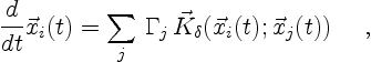
As discussed in section 3.2,
the convection is modeled by moving the vortices
according to the equation
To integrate (6.1), we used the fourth order Runge-Kutta time stepping scheme proposed by Blum [27].
Unfortunately, the cost of computing the velocity of all the vortices
using the summation (6.1)
is proportional to ![]() , where
, where ![]() is the number of vortices.
Such computational effort would be unrealistic for flows where
significant small-scale motion requires a fine vortex spacing,
in other words, large
is the number of vortices.
Such computational effort would be unrealistic for flows where
significant small-scale motion requires a fine vortex spacing,
in other words, large ![]() .
.
To solve this dilemma, `fast' algorithms were developed by,
among others, Greengard and Rokhlin [97] and
Carrier et al. [36], and independently by
Van Dommelen and Rundensteiner [233,240].
For the computations in this work the latter of these three schemes was
used; it seems to have been the first available scheme that
was solution adaptive [240],
but it can be noticeably slower than the first two schemes.
For all these schemes, the required amount of work is roughly
proportional to ![]() .
More recent variations have been proposed by a number of authors,
such as
[2,5,10,74,75].
.
More recent variations have been proposed by a number of authors,
such as
[2,5,10,74,75].
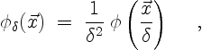
As explained in section 3.1,
the velocity field
![]() of a vortex is obtained by convolving the velocity field
of a vortex is obtained by convolving the velocity field
![]() of a point vortex
with a smoothing function
of a point vortex
with a smoothing function
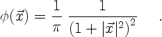
![]() which
is usually taken to be of the form
which
is usually taken to be of the form