5.9 A Summary of Separation of Variables

After the previous three examples, it is time to give a more general description of the method of separation of variables.

5.9.1 The form of the solution

Before starting the process, you should have some idea of the form of the solution you are looking for. Some experience helps here.

For example, for unsteady heat conduction in a bar of length $\ell$, with homogeneous end conditions, the temperature $u$ would be written

$$u(x,t) = \sum_n u_n(t) X_n(x)$$

where the $X_n$ are chosen eigenfunctions and the $u_n$ are computed Fourier coefficients of $u$. The separation of variables procedure allows you to choose the eigenfunctions cleverly.

For a uniform bar, you will find sines and/or cosines for the functions $X_n$. In that case the above expansion for $u$ is called a Fourier series. In general it is called a generalized Fourier series.

After the functions $X_n$ have been found, the Fourier coefficients $u_n$ can simply be found from substituting the expression above for $u$ in the given partial differential equation and initial conditions. (The boundary conditions are satisfied when you choose the eigenfunctions $X_n$.) If there are other functions in the partial differential equation or initial conditions, they too need to be expanded in a Fourier series.

If the problem was axially symmetric heat conduction through the wall of a pipe, the temperature would still be written

$$u(r,t) = \sum_n u_n(t) R_n(r)$$

but the expansion functions $R_n$ would now be found to be Bessel functions, not sines or cosines.

For heat conduction through a pipe wall without axial symmetry, still with homogeneous boundary conditions, the temperature would be written

$$u(r,\theta,t) = \sum_{n,i} u^i_n(r,t) \Theta^i_n(\theta) = \sum_{n,i} \sum_m u^i_{nm}(t) R_{nm}(r) \Theta^i_n(\theta)$$

where the eigenfunctions $\Theta^i_n$ turn out to be sines and cosines and the eigenfunctions $R_{nm}$ Bessel functions. Note that in the first sum, the temperature is written as a simple Fourier series in $\theta$, with coefficients $u_n$ that of course depend on $r$ and $t$. Then in the second sum, these coefficients themselves are written as a (generalized) Fourier series in $r$ with coefficients $u_{nm}$ that depend on $t$.

(For steady heat conduction, the coordinate ``$t$'' might actually be a second spatial coordinate. For convenience, we will refer to conditions at given values of $t$ as ``initial conditions'', even though they might physically really be boundary conditions.)

5.9.2 Limitations of the method

The problems that can be solved with separation of variables are relatively limited.

First of all, the equation must be linear. After all, the solution is found as an sum of simple solutions.

The partial differential equation does not necessarily have to be a constant coefficient equation, but the coefficients cannot be too complicated. You should be able to separate variables. A coefficient like $\sin(xt)$ in the equation is not separable.

Further, the boundaries must be at constant values of the coordinates. For example, for the heat conduction in a bar, the ends of the bar must be at fixed locations $x=0$ and $x=\ell$. The bar cannot expand, since then the end points would depend on time.

You may be able to find fixes for problems such as the ones above, of course. For example, the nonlinear Burger's equation can be converted into the linear heat equation. The above observations apply to straightforward application of the method.

5.9.3 The procedure

The general lines of the procedure are to choose the eigenfunctions and then to find the (generalized) Fourier coefficients of the desired solution $u$. In more detail, the steps are:

1. Make the boundary conditions for the eigenfunctions $X_n$ homogeneous
   
   For heat conduction in a bar, this means that if nonzero end temperatures or heat fluxes through the ends are given, you will need to eliminate these.
   
   Typically, you eliminate nonzero boundary conditions for the eigenfunctions by subtracting a function $u_0$ from $u$ that satisfies these boundary conditions. Since $u_0$ only needs to satisfy the boundary conditions, not the partial differential equation or the initial conditions, such a function is easy to find.
   
   If the boundary conditions are steady, you can try subtracting the steady solution, if it exists. More generally, a low degree polynomial can be tried, say $u_0=A+Bx+Cx^2$, where the coefficients are chosen to satisfy the boundary conditions.
   
   Afterwards, carefully identify the partial differential equation and initial conditions satisfied by the new unknown $v=u-u_0$. (They are typically different from the ones for $u$.)

2. Identify the eigenfunctions $X_n$
   
   To do this substitute a single term $T X$ into the homogeneous partial differential equation. Then take all terms involving $X$ and the corresponding independent variable to one side of the equation, and $T$ and the other independent variables to the other side. (If that turns out to be impossible, the partial differential equation cannot be solved using separation of variables.)
   
   Now, since the two sides of the equation depends on different coordinates, they must both be equal to some constant. The constant is called the eigenvalue.
   
   Setting the $X$-side equal to the eigenvalue gives an ordinary differential equation. Solve it to get the eigenfunctions $X_n$. In particular, you get the complete set of eigenfunctions $X_n$ by finding all possible solutions to this ordinary differential equation. (If the ordinary differential equation problem for the $X_n$ turns out to be a regular Sturm-Liouville problem of the type described in the next section, the method is guaranteed to work.)
   
   The equation for $T$ is usually safest ignored. The book tells you to also solve for the $T_n$, to get the Fourier coefficients $v_n$, but if you have an inhomogeneous partial differential equation, you have to mess around to get it right. Also, it is confusing, since the eigenfunctions $X_n$ do not have undetermined constants, but the coefficients $v_n$ do. It are the undetermined constants in $v_n$ that allow you to satisfy the initial conditions. They probably did not make this fundamental difference between the functions $X_n$ and the coefficients $u_n$ clear in your undergraduate classes.
   
   There is one case in which you do need to use the equation for the $T_n$: in problems with more than two independent variables, where you want to expand the $T_n$ themselves in a generalized Fourier series. That would be the case for the pipe wall without axial symmetry. Simply repeat the above separation of variables process for the partial differential equation satisfied by the $T_n$.
   
   
3. Find the coefficients
   
   Now find the Fourier coefficients $v_n$ (or $v_{nm}$ for three independent variables) by putting the Fourier series expansion into the partial differential equation and initial conditions.
   
   While doing this, you will also need to expand the inhomogeneous terms in the partial differential equation and initial conditions into a Fourier series of the same form. You can find the coefficients of these Fourier series using the orthogonality property described in the next section.
   
   You will find that the partial differential equation produces ordinary differential equations for the individual coefficients. And the integration constants in solving those equations follow from the initial conditions.
   
   

Afterwards you can play around with the solution to get other equivalent forms. For example, you can interchange the order of summation and integration (which results from the orthogonality property) to put the result in a Green's function form, etcetera.

5.9.4 More general eigenvalue problems

So far, the eigenvalue problems in the examples were of the form $X''=-\lambda X$. But you might get a different problem in other examples. Usually that produces a different orthogonality expression.

You can figure out what is the correct expression by writing your ordinary differential equation in the standard form of a Sturm-Liouville problem:

$$\fbox{$\displaystyle - p X'' - p'X' + q X = \lambda \bar {\rm r} X, $}$$

where $X(x)$ is the eigenfunction to be found and $p(x)>0$, $q(x)$, and $\bar {\rm r}(x)>0$ are given functions. The distinguishing feature is that the coefficient of the second, $X'$, term is the derivative of the coefficient of the first, $X''$ term.

Starting with an arbitrary second order linear ordinary differential equation, you can achieve such a form by multiplying the entire ordinary differential equation with a suitable factor.

The boundary conditions may either be periodic ones,

$$X(b) = X(a) \qquad X'(b) = X'(a),$$

or they can be homogeneous of the form

$$A X(a) + B X'(a) = 0 \qquad C X(b) + D X'(b) = 0,$$

where $A$, $B$, $C$, and $D$ are given constants. Note the important fact that a Sturm-Liouville problem must be completely homogeneous: $X=0$ must be a solution.

If you have a Sturm-Liouville problem, simply (well, simply ...) solve it. The solutions only exists for certain values of $\lambda$. Make sure you find all solutions, or you are in trouble. They will form an infinite sequence of `eigenfunctions', say $X_1(x)$, $X_2(x)$, $X_3(x)$, ... with corresponding `eigenvalues' $\lambda_1$, $\lambda_2$, $\lambda_3$, ... that go off to positive infinity.

You can represent arbitrary functions, say $f(x)$, on the interval $[a,b]$ as a generalized Fourier series:

$$f(x) = \sum_n f_n X_n(x).$$

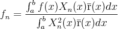
If you know $f(x)$, the orthogonality relation that gives the generalized Fourier coefficients $f_n$ is

$$f_n = \frac {\int_a^b f(x) X_n(x) \bar {\rm r}(x)\/dx} {\int_a^b X^2_n(x) \bar {\rm r}(x)\/dx}$$

Now you know why you need to write your Sturm-Liouville problem in standard form: it allows you to pick out the weight factor $\bar{\rm {r}}$ that you need to put in the orthogonality relation!