|
|
|
|
|
Next: 5.5 Finding the Green's function |
|
|
|
|
|
|
Next: 5.5 Finding the Green's function |
|
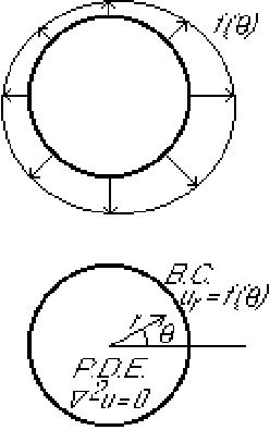
In this section the method of separation of variables will be applied to a problem in polar coordinates. The selected problem turns out to have two eigenfunctions for each eigenvalue other than the lowest.
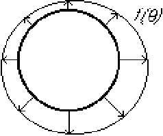
The problem is to find the ideal flow in a unit circle if the normal
(radial) velocity on the perimeter is known.
We will try to find a solution of this problem in the form
The reason to take the ![]() as the eigenfunctions and not
the
as the eigenfunctions and not
the ![]() is because separation of variables needs homogeneous boundary
conditions. The
is because separation of variables needs homogeneous boundary
conditions. The ![]() direction has an inhomogeneous boundary
condition
direction has an inhomogeneous boundary
condition
![]() at
at ![]() .
.
This follows the same procedures as in the first example. We
substitute a single term
![]() into the
homogeneous partial differential equation
into the
homogeneous partial differential equation
Now which ordinary differential equation gives us the Sturm-Liouville problem, and thus the
eigenvalues? Not the one for ![]() ;
; ![]() has an inhomogeneous
boundary condition on the perimeter
has an inhomogeneous
boundary condition on the perimeter ![]() . Eigenvalue problems must
be homogeneous; they simply don't work if anything is inhomogeneous.
. Eigenvalue problems must
be homogeneous; they simply don't work if anything is inhomogeneous.
We are in luck with
![]() however. The unknown
however. The unknown
![]() has ``periodic'' boundary conditions in the
has ``periodic'' boundary conditions in the
![]() -direction. If
-direction. If ![]() increases by an amount
increases by an amount ![]() ,
,
![]() returns to exactly the same values as before: it is a
``periodic function'' of
returns to exactly the same values as before: it is a
``periodic function'' of ![]() . Periodic boundary conditions
are homogeneous: the zero solution satisfies them. After all, zero
remains zero however many times you go around the circle.
. Periodic boundary conditions
are homogeneous: the zero solution satisfies them. After all, zero
remains zero however many times you go around the circle.
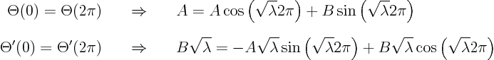
The Sturm-Liouville problem for ![]() is:
is:
Pretend that we do not know the solution of this Sturm-Liouville problem!
Write the characteristic equation of the ordinary differential equation:
Since ![]() :
:
Boundary conditions:
We will be lazy and try to do the cases of positive and negative
![]() at the same time. For positive
at the same time. For positive ![]() , the cleaned-up
solution is
, the cleaned-up
solution is
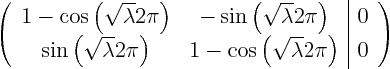
Lets write down the boundary conditions first:
These two equations are a bit less simple than the ones we saw so far.
Rather than directly trying to solve them and make mistakes, this time
let us write out the augmented matrix of the system of equations for
![]() and
and ![]() :
:
If ![]() is negative,
is negative,
![]() which is always greater
than one for nonzero
which is always greater
than one for nonzero ![]() .
.
For the found eigenvalues, the system of equations for ![]() and
and ![]() becomes:
becomes:
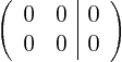
We had this situation before with eigenvector in the case of double
eigenvalues, where an eigenvalue gave rise two linearly independent
eigenvectors. Basically we have the same situation here: each
eigenvalue is double. Similar to the case of eigenvectors of
symmetric matrices, here we want two linearly independent, and more
specifically, orthogonal eigenfunctions. A suitable pair is
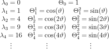
We can now tabulate the complete set of eigenvalues and eigenfunctions
now as:
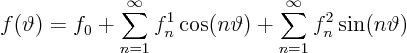
We will again expand all variables in the problem in a Fourier series.
Let's start with the function ![]() giving the outflow through
the perimeter.
giving the outflow through
the perimeter.
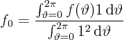
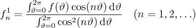
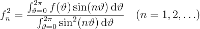
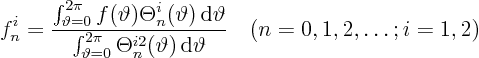
Since ![]() is supposedly known, we should again be able to find
its Fourier coefficients using orthogonality. The formulae
are as before.
is supposedly known, we should again be able to find
its Fourier coefficients using orthogonality. The formulae
are as before.
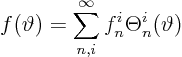
Since I hate typing big formulae, allow me to write the Fourier series
for ![]() much more compactly as
much more compactly as
Next, let's write the unknown
![]() as a compact Fourier
series:
as a compact Fourier
series:
We put this into partial differential equation
![]() :
:


We get the following ordinary differential equation for ![]() :
:
Fortunately, we have seen this one before: it is the Euler equation.
You solved that one by changing to the logarithm of the independent
variable, in other words, by rewriting the equation in terms of
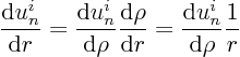
![\begin{displaymath}
\frac{{\rm d}^2 u^i_n}{{\rm d}r^2} =
\frac{{\rm d}}{{\rm...
...ght] \frac1r
- \frac{{\rm d}u^i_n}{{\rm d}\rho} \frac1{r^2}
\end{displaymath}](img1058.gif)
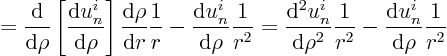
The ordinary differential equation becomes in terms of ![]() :
:
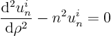
Now both ![]() as well as
as well as ![]() are infinite when
are infinite when
![]() . But that is in the middle of our flow region, and the
flow is obviously not infinite there. So from the `boundary
condition' at
. But that is in the middle of our flow region, and the
flow is obviously not infinite there. So from the `boundary
condition' at ![]() that the flow is not singular, we conclude that
all the
that the flow is not singular, we conclude that
all the ![]() -coefficients must be zero. Since
-coefficients must be zero. Since ![]() , all coefficients
are of the form
, all coefficients
are of the form ![]() , including the one for
, including the one for ![]() .
.
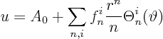
Hence our solution can be more precisely written
Next we expand the boundary condition
![]() at
at ![]() in a Fourier series:
in a Fourier series:
For ![]() , we see immediately that
, we see immediately that ![]() can be anything, but we need
can be anything, but we need
![]() for a solution to exist! According to the orthogonality
relationship for
for a solution to exist! According to the orthogonality
relationship for ![]() , this requires:
, this requires:
For nonzero ![]() :
:
Let's summarize our results, and write the eigenfunctions out in terms of the individual sines and cosines.
Required for a solution is that:
Then: