|
|
|
|
|
Next: 6. Fourier Transforms [None] |
|
This example addresses a much more complex case. It involves three independent variables and eigenfunctions that turn out to be Bessel functions.
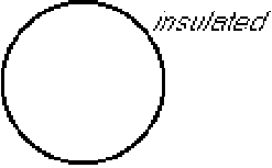
Find the unsteady heat conduction in a disk if the perimeter is
insulated. The initial temperature is given.
We will solve using separation of variables in the form
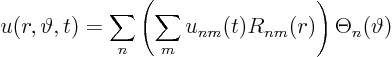
Let's start trying to get rid of one variable first. We might try
a solution of the form
Try again, this time
So we have a Sturm-Liouville problem for ![]() :
:
Like we did in 7.38, in order to cut down on writing, we will indicate
those eigenfunctions compactly as ![]() , where
, where
![]() and
and
![]() .
.
So we can concisely write
We must go one step further: in addition we need to expand each
Fourier coefficient ![]() in a generalized Fourier series in
in a generalized Fourier series in ![]() :
:
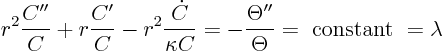
Now, if you put a single term of the form
![]() into the homogeneous partial differential equation, you get
into the homogeneous partial differential equation, you get
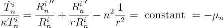
So we get a Sturm-Liouville problem for ![]() with eigenvalue
with eigenvalue ![]()
Unfortunately, the ordinary differential equation above is not a constant coefficient one, so we
cannot write a characteristic equation. However, we have seen the
special case that ![]() before, 7.38. It was a Euler equation.
We found in 7.38 that the only solutions that are regular at
before, 7.38. It was a Euler equation.
We found in 7.38 that the only solutions that are regular at ![]() were found to be
were found to be ![]() . But over here, the only one of that form
that also satisfies the boundary condition
. But over here, the only one of that form
that also satisfies the boundary condition ![]() at
at ![]() is the
case
is the
case ![]() . So, for
. So, for ![]() , we only get a single eigenfunction
, we only get a single eigenfunction
For the case ![]() , the trick is to define a stretched
, the trick is to define a stretched ![]() coordinate
coordinate ![]() as
as

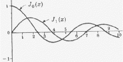
Now we need to apply the boundary conditions. Now if you look up the
graphs for the functions ![]() , or their power series around the
origin, you will see that they are all singular at
, or their power series around the
origin, you will see that they are all singular at ![]() . So,
regularity at
. So,
regularity at ![]() requires
requires ![]() .
.
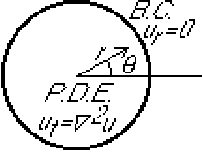
The boundary condition at the perimeter is
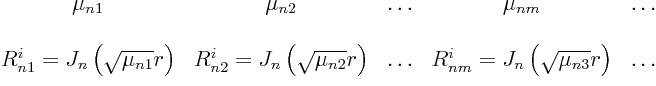
So the ![]() -eigenvalues and eigenfunctions are:
-eigenvalues and eigenfunctions are:
In case of negative ![]() , the Bessel function
, the Bessel function ![]() of imaginary
argument becomes a modified Bessel function
of imaginary
argument becomes a modified Bessel function ![]() of real argument,
and looking at the graph of those, you see that there are no
solutions.
of real argument,
and looking at the graph of those, you see that there are no
solutions.
We again expand all variables in the problem in generalized Fourier
series:
Let's start with the initial condition:
To find the Fourier coefficients ![]() , we need orthogonality
for both the
, we need orthogonality
for both the ![]() and
and ![]() eigenfunctions. Now the ordinary differential equation for the
eigenfunctions. Now the ordinary differential equation for the
![]() eigenfunctions was in standard form,
eigenfunctions was in standard form,
As a result, our orthogonality relation for the Fourier coefficients
of initial condition
![]() becomes
becomes
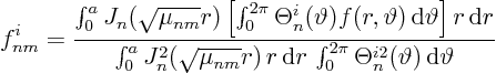
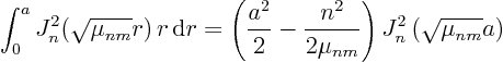
The ![]() -integral in the denominator can be worked out using Schaum's
Mathematical Handbook 24.88/27.88:
-integral in the denominator can be worked out using Schaum's
Mathematical Handbook 24.88/27.88:
Hence, while akward, there is no fundamental problem in evaluating as
many ![]() as you want numerically. We will therefor consider
them now ``known''.
as you want numerically. We will therefor consider
them now ``known''.
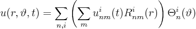
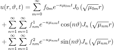
Next we expand the desired temperature in a generalized Fourier series:
Put into partial differential equation
![]() :
:
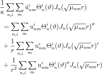
Because of the SL equation satisfied by the ![]() :
:

Because of the SL equation satisfied by the ![]() :
:
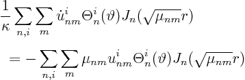
Hence the ordinary differential equation for the Fourier coefficients is:
At time zero, the series expansion for ![]() must be the same as the
one for the given initial condition
must be the same as the
one for the given initial condition ![]() :
:
Find the set
![]() of positive stationary points of the
Bessel functions
of positive stationary points of the
Bessel functions ![]() ,
, ![]() and add
and add ![]() .
.
Find the generalized Fourier coefficients of the initial condition:
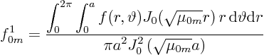
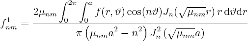
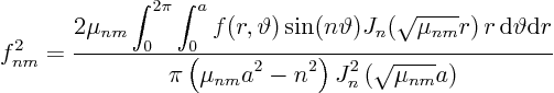
Then:
That was not too bad!