|
|
|
To: 8.2.7 Comparison with boundary layer theory |
In this section we want to discuss a question that has not received
sufficient attention in the past; the question when the vorticity is small
enough that a numerical computation can neglect it. Of course, since the
incompressible Navier-Stokes equations have elliptic properties, for all
nonzero times the vorticity field extends all the way to infinity. But the
vorticity well above the boundary layers is exponentially small, and is
neglected beyond some point in almost any scheme. For example, a finite
difference scheme may impose a condition of zero vorticity or zero
vorticity flux at some cutoff line well above the viscous region. In a
pressure-velocity formulation, meaningful information about the vorticity
no longer exists when the numerical errors in the velocity differences
exceed velocity differences
due to the vorticity. As we explained in subsection
6.2.5, in our own computations, as well as in various other
vortex computations, the generation of excessive numbers of
vortices with exponentially small strength
is prevented by not diffusing vortices if their
strength is less than some very small ``cutoff circulation"
![]() .
.
However, as we also pointed out in subsection 6.2.5, Van Dommelen & Shen [239] warned that this may be dangerous. These authors studied the boundary layer flow at the rear stagnation point, and discovered that its behavior for long times is completely determined by the exponentially small velocities above the boundary layer. It suggests that great care must be taken to select a value of the cutoff circulation, since it can destroy essential information. This is especially likely for flows at high Reynolds numbers since the exact solution of Van Dommelen & Shen [239] is being approached more closely for increasing Reynolds number. The warning applies to any numerical scheme, since it is due to the physics of the flow itself.
To show that the warning is highly relevant, we will now present the
effect of the value of
![]() .
.
 |
 |
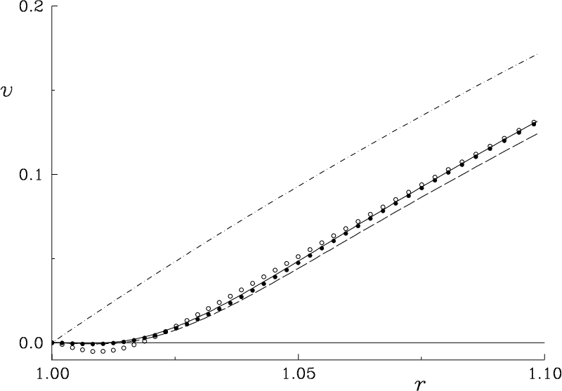
One clear effect of the cut-off circulation on the computed velocity
is shown in figure 8.31.
The figure shows the radial velocity
along the rear symmetry axis at an early time ![]() .
The computed velocity
for
.
The computed velocity
for
![]() is in excellent
agreement with that
of the second-order boundary layer theory
of Van Dommelen & Shankar (unpublished).
However, for a higher value
is in excellent
agreement with that
of the second-order boundary layer theory
of Van Dommelen & Shankar (unpublished).
However, for a higher value
![]() ,
there are significant errors; for example,
the flow reverses earlier as indicated by the negative velocity.
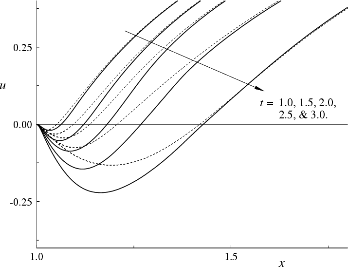
For later times, figure 8.32 shows that the
computed velocity fields obtained using
,
there are significant errors; for example,
the flow reverses earlier as indicated by the negative velocity.
For later times, figure 8.32 shows that the
computed velocity fields obtained using
![]() and
and
![]() differ even more widely than at
differ even more widely than at ![]() .
.
 |
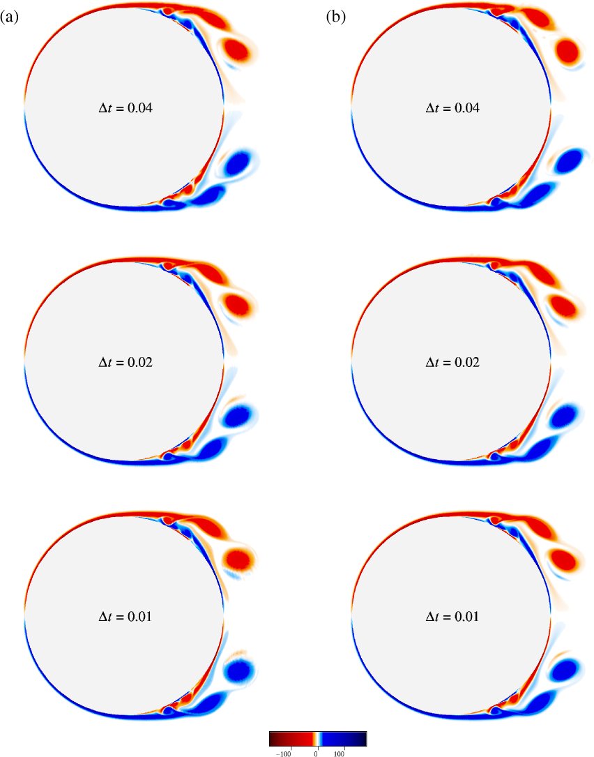 |
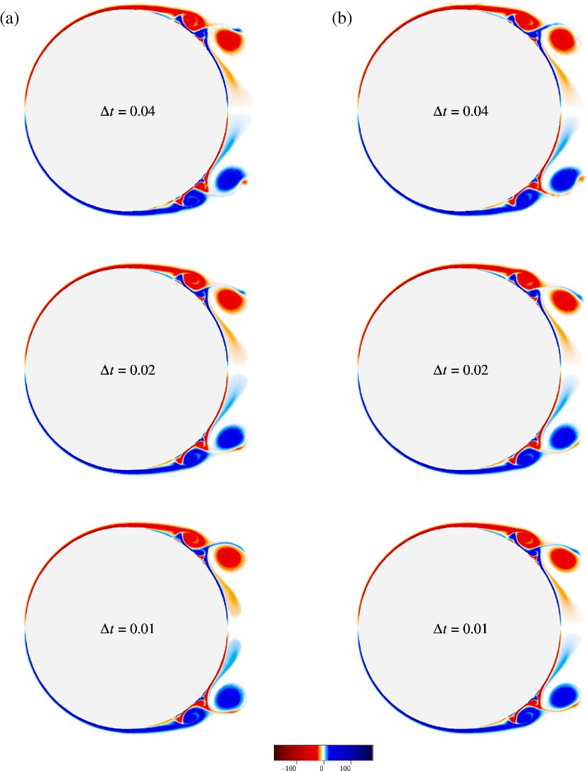
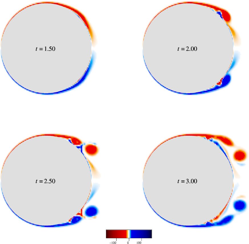
Figures 8.33 and 8.34
show the effect of the cut-off circulation on the computed
vorticity fields at two different times ![]() and
and ![]() .
The figures show that for
.
The figures show that for
![]() (lower cut-off) ,
the computed vorticity fields converge as the time step
(lower cut-off) ,
the computed vorticity fields converge as the time step
![]() is reduced.
However, for a higher value
of
is reduced.
However, for a higher value
of
![]() , the computed vorticity fields
do not converge as the time step is reduced.
The reason that the vorticity fields do not converge is the following:
As the time step is reduced, the number of vortices increases
inversely proportional to the time step.
As the number of vortices increases,
the average circulation of a vortex is reduced, and hence the same
cut-off circulation neglects more of the vorticity field.
This evidenced by comparing the time steps
, the computed vorticity fields
do not converge as the time step is reduced.
The reason that the vorticity fields do not converge is the following:
As the time step is reduced, the number of vortices increases
inversely proportional to the time step.
As the number of vortices increases,
the average circulation of a vortex is reduced, and hence the same
cut-off circulation neglects more of the vorticity field.
This evidenced by comparing the time steps ![]() and
and
![]() for the larger cutoff in figure 8.33
and 8.34. The larger time step is in much better
agreement with the converged data for the smaller cutoff. Since the time
step change is equivalent to an equivalent change in
for the larger cutoff in figure 8.33
and 8.34. The larger time step is in much better
agreement with the converged data for the smaller cutoff. Since the time
step change is equivalent to an equivalent change in
![]() by
only a factor 2, we believe our factor 10 reduction in
by
only a factor 2, we believe our factor 10 reduction in
![]() for our final results should be more than enough. This is further supported
by the comparisons with the analytical solution in figures
8.13 and 8.31.
However, detailed convergence studies would need to be conducted to
clarify the precise limits.
for our final results should be more than enough. This is further supported
by the comparisons with the analytical solution in figures
8.13 and 8.31.
However, detailed convergence studies would need to be conducted to
clarify the precise limits.
 |
Similarly, the computations [117,119,208]
based on the
particle strength exchange scheme also use a cut-off vorticity parameter;
the particles are eliminated from the computations if their vorticity
values fall below a chosen cut-off vorticity value.
Shiels's [208]
preliminary computation
of the impulsively started cylinder flow at ![]() shows that
the computed vorticity fields are significantly affected if the
cut-off vorticity is chosen to be too high;
compare the vorticity fields in figure 8.35
computed using a cut-off vorticity is
shows that
the computed vorticity fields are significantly affected if the
cut-off vorticity is chosen to be too high;
compare the vorticity fields in figure 8.35
computed using a cut-off vorticity is ![]() and that of
figure 8.22(a) computed using a cut-off vorticity
and that of
figure 8.22(a) computed using a cut-off vorticity
![]() .
Notice that his computed vorticity field in figure 8.35
at
.
Notice that his computed vorticity field in figure 8.35
at ![]() is remarkably similar to our unconverged
vorticity field in figure 8.34(a)
corresponding to
is remarkably similar to our unconverged
vorticity field in figure 8.34(a)
corresponding to ![]() .
The `blockiness' in the figure 8.35 is simply due to the
coarseness of the mesh he used to plot the vorticity and
not due to the computation itself.
In his computation, the
time step is
.
The `blockiness' in the figure 8.35 is simply due to the
coarseness of the mesh he used to plot the vorticity and
not due to the computation itself.
In his computation, the
time step is
![]() ; and the Gaussian kernel size is
1.1 times the average spacing between the particles. The
number
of particles in his computation is
236,000 at
; and the Gaussian kernel size is
1.1 times the average spacing between the particles. The
number
of particles in his computation is
236,000 at ![]() , 380,000 at
, 380,000 at ![]() , and 543,000 at
, and 543,000 at ![]() .
.
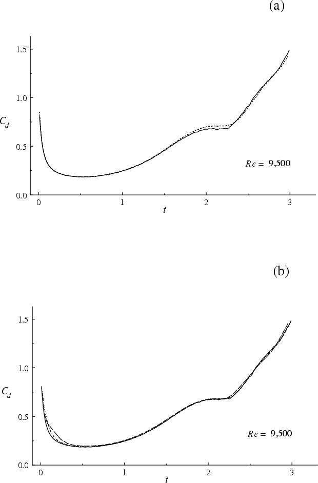 |
The computed drag values are also affected by the cut-off
circulation, figure 8.36(a).
This figure indicates that seemingly small
differences between drag curves could really mean
significant differences in the respective vorticity fields.
Notice that the computed drag obtained using ![]() is in
much better agreement with the converged drag values,
figure 8.36(b). As before, it indicates that our final
cutoff
is in
much better agreement with the converged drag values,
figure 8.36(b). As before, it indicates that our final
cutoff ![]() should be sufficient.
should be sufficient.