|
|
|
To: 8.2 Impulsively translated cylinder |
 |
The first flow we consider is the Stokes flow (![]() ) over a circular
cylinder impulsively set into an uniform rotation about its axis.
The boundary condition on the cylinder surface is the no-slip
condition (2.5); the vorticity vanishes
far away from the cylinder surface.
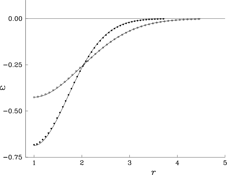
Figure 8.1 shows that the computed vorticity
distributions agree well with the finite difference solutions.
) over a circular
cylinder impulsively set into an uniform rotation about its axis.
The boundary condition on the cylinder surface is the no-slip
condition (2.5); the vorticity vanishes
far away from the cylinder surface.
Figure 8.1 shows that the computed vorticity
distributions agree well with the finite difference solutions.
 |
The second flow we consider is the Stokes flow around a circular
cylinder set into periodic rotational oscillations about its axis.
This periodic motion is taken to be
![]() ; where
; where ![]() is the
viscous time
is the
viscous time ![]() .
The boundary condition on the cylinder surface is the no-slip
condition (2.5), while the vorticity vanishes
far away from the cylinder surface.
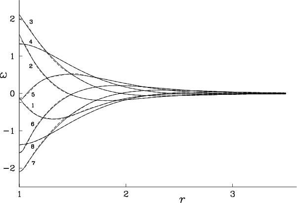
Figure 8.2 shows the vorticity field along a radial line at
different times during the first time period of oscillation.
The numbers 1 to 8 close to the curves indicate the relative phase of the
oscillation; they are
.
The boundary condition on the cylinder surface is the no-slip
condition (2.5), while the vorticity vanishes
far away from the cylinder surface.
Figure 8.2 shows the vorticity field along a radial line at
different times during the first time period of oscillation.
The numbers 1 to 8 close to the curves indicate the relative phase of the
oscillation; they are ![]() of the time period apart.
Initially a Stokes layer develops on the cylinder surface.
For large times, the flow becomes periodic due to the
periodicity of the boundary condition; our computation shows that
the flow becomes periodic by the end of one time period of oscillation.
The exact periodic solution
derived by McLachlan
[151] and Winny
[248] was used to check the periodic solutions computed
using the finite difference method.
The redistribution solution clearly
follows the transient solution computed using
finite differences, and reaches the periodic solution.
of the time period apart.
Initially a Stokes layer develops on the cylinder surface.
For large times, the flow becomes periodic due to the
periodicity of the boundary condition; our computation shows that
the flow becomes periodic by the end of one time period of oscillation.
The exact periodic solution
derived by McLachlan
[151] and Winny
[248] was used to check the periodic solutions computed
using the finite difference method.
The redistribution solution clearly
follows the transient solution computed using
finite differences, and reaches the periodic solution.
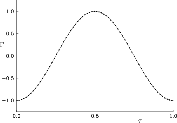 |
It may be noted, however, that the vorticity values on the cylinder surface show deviations from the finite difference solution. These deviations are not due to the vorticity redistribution method itself, but arise from evaluating the vorticity using smoothing functions as discussed in subsection 6.2.6. In fact, figure 8.3 shows that the total circulation computed by the vorticity redistribution method is in excellent agreement with the finite difference solution. This must mean that the deviations in figure 8.2 are only artificial. They can be removed by a more elaborate evaluation procedure near the wall (subsection 6.2.6). The vorticity distributions in the above two flows are axisymmetric and our computations reproduced that symmetry very well even though it was not explicitly enforced.
The excellent agreement of our two-dimensional redistribution results with the effectively exact one-dimensional finite difference solution provides strong support for the numerical implementation of the boundary conditions discussed in section 6.3. However, for these two-dimensional axisymmetric flows, the convection term in the vorticity equation vanishes identically. To test our method also for flows in which convection is not trivial, we compute the flow over an impulsively translated circular cylinder in the next section.