|
|
|
To: 6.2.4 Merging vortices |
The numerical technique of the previous two subsections 6.2.1 and 6.2.2 will find a positive solution to the redistribution equations as long as one exists. A solution does not necessarily exist, however. In that case, new vortices with zero circulation are added until a positive solution does become possible.
There are various reasons why a solution may not exist. For example, the number of vortices in the neighborhood may be less than the chosen number of redistribution equations. First-order accuracy requires at least six vortices, and this number increases for higher order.
Further
the neighborhood radius may be too small for the desired order
of accuracy ![]() .
According to an estimate derived in Appendix A, the scaled neighborhood
radius
.
According to an estimate derived in Appendix A, the scaled neighborhood
radius ![]() must be at least
must be at least ![]() , with
, with ![]() the even integer
the even integer
![]() or
or ![]() .
For first or second-order accuracy, this requires a minimum value
.
For first or second-order accuracy, this requires a minimum value ![]() .
For third-order accuracy or higher,
the vortices should also not be spaced too far apart;
the scaled spacing cannot exceed
.
For third-order accuracy or higher,
the vortices should also not be spaced too far apart;
the scaled spacing cannot exceed ![]()
At the outer edge of the region containing the vortices, a solution always requires new vortices. According to an estimate derived in Appendix A, the vortex region must expand by a finite scaled distance in each direction.
On the other hand, under reasonable conditions positive solutions
to the redistribution equations do exist.
For example, a standard five-point explicit finite difference formula
with
![]() gives a second-order positive solution as long as
gives a second-order positive solution as long as ![]() is at least
the minimum value 2 mentioned above.
Similarly a fourth-order solution exists if
is at least
the minimum value 2 mentioned above.
Similarly a fourth-order solution exists if ![]() is at least
is at least ![]() ,
Appendix A.
,
Appendix A.
More generally, there is always a finite
scaled neighborhood radius ![]() for which the existence of a positive
solution is assured, provided only that are no `holes' in the distribution
of the vortices that exceed some finite scaled size
for which the existence of a positive
solution is assured, provided only that are no `holes' in the distribution
of the vortices that exceed some finite scaled size ![]() .
This is shown in Appendix A; however, it does not give values for
.
This is shown in Appendix A; however, it does not give values for ![]() and
and ![]() .
.
In our first-order computations,
we chose the redistribution radius ![]() , which
is well above the minimum value 2 for which a positive solution
becomes possible.
The reason is that the minimum value requires vortices placed at
optimum positions.
For a larger radius, a positive solution may be found for more
general vortex placings.
, which
is well above the minimum value 2 for which a positive solution
becomes possible.
The reason is that the minimum value requires vortices placed at
optimum positions.
For a larger radius, a positive solution may be found for more
general vortex placings.
One question of concern is where to place newly created vortices.
Van Dommelen [235] showed in one dimension that
if the computation starts with a single vortex
and new vortices are added at scaled distances ![]() , the fourth-order
accurate finite difference scheme is obtained.
Based on this observation, we adopted the strategy that if no positive
solution can be found for a certain vortex, a new vortex is added at a
scaled distance
, the fourth-order
accurate finite difference scheme is obtained.
Based on this observation, we adopted the strategy that if no positive
solution can be found for a certain vortex, a new vortex is added at a
scaled distance ![]() from the considered vortex.
The angular location of the new vortex is chosen among 12 possible
positions spaced 30 degrees apart, by maximizing the distance between
the new vortex and the existing vortices.
from the considered vortex.
The angular location of the new vortex is chosen among 12 possible
positions spaced 30 degrees apart, by maximizing the distance between
the new vortex and the existing vortices.
This procedure worked well in practice, but it is certainly not unique. For example, Van Dommelen showed that the new vortices may also be placed at random positions without apparent ill effects. However, our procedure has some advantages. It will always succeed: a positive solution is assured as soon as the points of a five-point finite difference stencil have been filled. It also tends to fill up the holes in the distribution of the vortices. Since the newly added vortices are located away from the edge of the redistribution region, it takes a finite time before they can convect out of it.
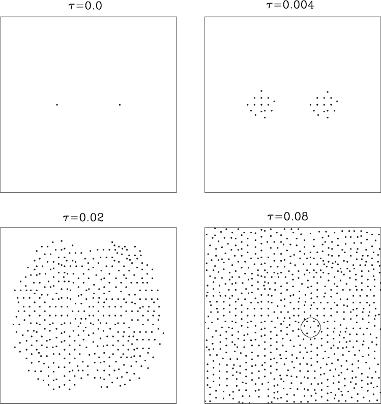 |
Figure 6.1 shows the increase in the number of vortices for an example computation. The computation is the Stokes flow starting from two concentrated, counter-rotating vortices. It is found that our strategy of placing new vortices increases the vortex density initially until it fills up the `holes' in the distribution. When a certain vortex density is reached, the distribution becomes steady. For example, the region shown for the final time in figure 6.1 is unchanged at double that time.
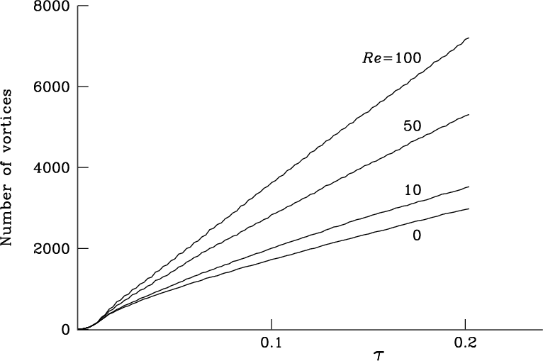
As shown in figure 6.2, the total number of vortices in the computation does continue to grow. The reason is that new vortices continue to be added at the edge of the distribution. In fact, since the region containing vorticity continues to grow linearly with time, ideally the number of vortices should also grow linearly.
However, it was noted above that redistribution must expand the region containing the vortices by a scaled distance that does not depend on time. This would lead to a number of vortices that grows quadratically with time. It would lead to large amounts of vortices with exponentially small strengths at large distances. To prevent this growth, we do not redistribute a vortex if its strength is below a small ``cut-off" value. Using this restriction, figure 6.2 shows that the growth in the number of vortices is indeed quite linear. Yet one discovery made in this thesis is that the effect of a cut-off that is not small enough can be disastrous under certain circumstances. This is discussed in subsection 6.2.5.
Convection introduces a further complication. Even if a vortex can be redistributed at a given time, after a finite time convection can move the vortices to locations for which a positive solution may no longer exist. In that case new vortices must be added. This can happen even though incompressibility ensures that the average vortex density does not change. The reason is that vortices might approach closely, which allows holes in the vortex distribution to form even though in principle there are enough vortices to fill those.
|
As an example, figure 6.3 shows the evolution of the vortex distribution at Reynolds number 50, when there are very strong convection effects. While we always add new vortices in the biggest hole we can find locally, it is seen that convection has caused some vortices to approach closely. As a result, the number of vortices in a typical redistribution radius, shown as a circle, has increased compared to the case of no convection in figure 6.1. Figure 6.2 shows the increase in the total number of vortices with Reynolds number.
The additional vortices require increased computational resources. It also raises the more fundamental question whether the number of vortices within a redistribution distance remains finite. This requires a total number of vortices that increases linearly with the inverse of the time-step. Table 6.1 verifies this requirement at Reynolds number 50.
In the next subsection we will discuss ways to reduce the additional vortices caused by convection effects.