main

% Hyperelastic: Nonaffine model
% Viscoelastic: Linear
close all; clear all; clc;

The following code estimates hyperelastic and nonlinear viscoelastic parameters for a single stretch rate of the dielectric elastomer VHB 4910 made by 3M. Details describing the constitutive modeling framework is given in

Miles, P., Hays, M., Smith, R., Oates, W., "Bayesian Uncertainty Analysis of Finite Deformation Viscoelasticity," Mechanics of Materials, v. 91(1), p. 35-49, 2015.

Key details associated with the hyperelastic energy, entropy generation function, and associated parameters estimated using Bayesian statistics is given as follows.

We first introduce a Helmholtz energy density function that includes conventional hyperelasticity that depends on deformation and an additional energy density that quantifies evolution of internal state variables that are not conserved. The total Helmholtz free energy density is

$\psi = \psi_{\infty}(F_{iK}) + \Upsilon(F_{iK},\Gamma_{iK})$

where $\psi_{\infty}$ is the hyperelastic energy function which only depends on the deformation gradient ( $F_{iK}$ ) and $\Upsilon$ is an energy density that defines coupling with non-conserved internal state variables ( $\Gamma_{iK}$ ). The deformation gradient and internal state tensors use conventional indicial notation with $i,K=1,2,3$ .

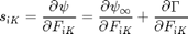
The total nominal stress, which is our quantity of interest (QoI) in the Bayesian calibration problem, is

$s_{iK} = \frac{\partial \psi}{\partial F_{iK}} = \frac{\partial \psi_{\infty}}{\partial F_{iK}} + \frac{\partial \Gamma}{\partial F_{iK}}$

It is important to note that we include incompressibility within $\frac{\partial \psi_{\infty}}{\partial F_{iK}}$ but do not explicitly define it here.

The reversible stress, independent of $\Gamma_{iK}$ is obtained from a non-affine hyperlastic energy function

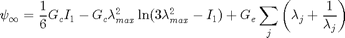
$\psi_{\infty} = \frac{1}{6}G_c I_1 - G_c \lambda_{max}^2 \ln(3\lambda_{max}^2 - I_1) + G_e \sum_j \left(\lambda_j + \frac{1}{\lambda_j}\right)$

where the first invariant is 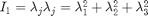$I_1 = \lambda_j \lambda_j = \lambda_1^2 + \lambda_2^2 + \lambda_3^2$ and $\lambda_j$ is the stretch in the principle directions (eigenvalues of $F_{iK}$ ). The unknown material parameters include the crosslink modulus $G_c$ , the entanglement modulus $G_e$ and the maximum stretch of a representative volume element $\lambda_{max}$ . This model was developed by Davidson and Goulbourne (see reference within Miles et al.).

Two different energy functions for $\Upsilon$ have been considered previously. We have either assumed the losses due to the internal state follow a quadratic dependence on the difference between the deformation gradient $F_{iK}$ and the internal state tensor $\Gamma_{iK}$ or assume $\Upsilon$ is proportional to the hyperelastic energy function. The former we call linear viscoelasticity and the latter we call nonlinear viscoelasticity. For simplicity, we implement the linear viscoelastic model here which requires

$\Upsilon = \frac{\gamma}{2}(F_{iK} - \Gamma_{iK})(F_{iK} - \Gamma_{iK})$

where $\gamma$ is another unknown material parameter.

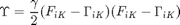
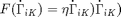
We must also introduce an additional equation to solve for $\Gamma_{iK}$ . This is accomplished using the second law of thermodynamics. Ultimately, a positive definite entropy generation function must be introduced. This function is defined to depend on the time rate of change of $\Gamma_{iK}$ according to

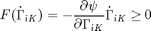
$F(\dot{\Gamma}_{iK}) = -\frac{\partial \psi}{\partial \Gamma_{iK}} \dot{\Gamma}_{iK} \ge 0$

where the middle relation is derived from the Clausius-Duhem inequality. The entropy generation function $F(\dot{\Gamma}_{iK})$ is assumed to be a quadratic function which assumes slow enough rates such that higher order terms are negligible. It is defined by

$F(\dot{\Gamma}_{iK}) = \eta \dot{\Gamma}_{iK}) \dot{\Gamma}_{iK})$

where $\eta$ is an unknown material parameter.

In summary, the Clausius-Duhem equation is solved simultaneously with the total nominal stress equation where the model input is the principle stretch. By assuming incompressibility, the principle stretch in the direction of uniaxial extension is prescribed while the two orthogonal stretches are solved from the incompressibility constraint.

The model parmeters obtained through the Bayesian calibration include

$\theta = [G_c, \lambda_{max}, G_e, \gamma, \eta, \beta]$

Note that the first three model parameters should be independent of the stretch rate. Here all parameters are identified from a single stretch rate. More details on different methods to independently determine the rate independent and rate dependent (viscoelastic) parameters is given in the paper by Miles et al. listed above.

addpath('mcmcstat');
addpath('Data_Files');

% -------------------------------------------------------------------------
%  Load Files
load('Experimental_Data_VHB_4910_Stretch_Rate_67.mat');

%  Generate data structure for mcmcrun
data.xdata = stretch;  % [-] - measure of deformation
data.ydata = stress;   % [kPa] - experimental stress
data.dta = dta;        % [s] - time step between each sampled point
data.ind = ind;        % [-] - index required when looking at multiple data sets.

The material parameter initial guesses for $\theta = [G_c, \lambda_{max}, G_e, \gamma, \eta, \beta]$ are defined here using kPa units.

Gc = 5.52;     % [kPa]
lam_max = 4.3; % [-]
Ge = 5.5;      % [kPa]
gamma = 110;   % [kPa]
eta = 550;     % [kPa*s];
beta = 4.4;    % [-];

% Define initial guesses and parameter upper and lower bounds
IP = [
    Gc           %G_c [kPa]
    lam_max      % max stretch [-]
    Ge           % G_e [kPa]
    gamma        % gamma - [kPa]
    eta         % eta   - [kPa*s]
    beta         % beta  - [-]
    ];

Lims = [ %      LL          UL
    1.00E-06	1.00E+09    % G_c
    1.00E-06	1.00E+09    % lam_max
    1.00E-06	1.00E+09    % G_e
    1.00E-06	1.00E+09    % gamma
    1.00E-06	1.00E+09    % eta
    1.00E-06	1.00E+09    % beta
    ];

LL = Lims(:,1); UL = Lims(:,2);

% -------------------------------------------------------------------------
% Define Parameter Cell Array
params =  {
    {'G_c',            IP(1), LL(1), UL(1)}
    {'\lambda_{max}',  IP(2), LL(2), UL(2)}
    {'G_e',            IP(3), LL(3), UL(3)}
    {'\gamma',         IP(4), LL(4), UL(4)}
    {'\eta',           IP(5), LL(5), UL(5)}
    {'\beta',          IP(6), LL(6), UL(6)}
    };

The key Bayesian Markov Chain Monte Carlo (MCMC) model settings are defined and executed in this section.

ssfun = @ss_func; % (theta,data)
model.ssfun=ssfun; % Sum-of-Squares function
model.S20 = 1;
model.N0  = 1;
model.N = size(data.xdata,1);
options.nsimu = 5e4;    % user defined number of simulations to run
options.updatesigma = 1;

% -------------------------------------------------------------------------
% MCMC
[results, chain, s2chain, sschain] = mcmcrun(model, data, params, options);

Sampling these parameters:
name   start [min,max] N(mu,s^2)
G_c: 5.52 [1e-06,1e+09] N(0,Inf)
\lambda_{max}: 4.3 [1e-06,1e+09] N(0,Inf)
G_e: 5.5 [1e-06,1e+09] N(0,Inf)
\gamma: 110 [1e-06,1e+09] N(0,Inf)
\eta: 550 [1e-06,1e+09] N(0,Inf)
\beta: 4.4 [1e-06,1e+09] N(0,Inf)

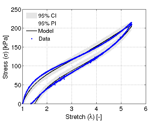
Once the results and chains have been quantified. The statistics are used to generate prediction/credible intervals by propogating the error through model.

modelfun = @(d,th) vhb_model(th,d);
nsample = 500;
out = mcmcpred(results, chain, s2chain, data, modelfun, nsample);

% -------------------------------------------------------------------------
% Calculate Error
[ss, sigma_model] = ss_func(results.mean, data);
l2norm = norm((sigma_model - data.ydata), 2);
e_mcmc = ss/length(data.ydata);

% Display chain statistics
fprintf('L2-norm: %4.2f\n', l2norm);
fprintf('e_mcmc: %4.2f\n', e_mcmc);
chainstats(chain)

% -------------------------------------------------------------------------
% Plotting command shortcuts
FS = 'FontSize'; LW = 'LineWidth'; MS = 'MarkerSize';

% -------------------------------------------------------------------------

L2-norm: 197.41
e_mcmc: 30.54
MCMC statistics, nsimu = 50000

      mean         std      MC_err         tau      geweke
----------------------------------------------------------
    6.2472      1.0592     0.15683        1272     0.96579
     4.331    0.057684   0.0048689      384.64     0.98634
    6.5697      1.1656     0.16705      1251.4     0.98933
    93.333      10.355      1.4343      1195.6     0.98456
     624.4      71.696      10.626      1220.6     0.94105
    3.3644     0.74631     0.11312      1222.3     0.94888
----------------------------------------------------------

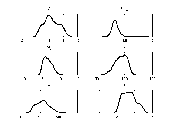
Density Panel displays the distribution of each parameter samples. It gives some indication to the likelihood of each parameter being a certain value. Additionally, narrow distributions imply strong dependence on the parameter being that value, whereas broad distributions imply a lack of significance.

figure(1)
mcmcplot(chain,[],results,'denspanel', 2);

% -------------------------------------------------------------------------

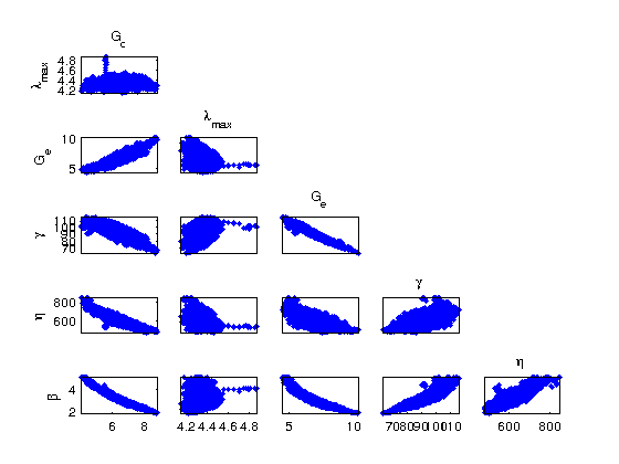
Pairs displays the correlations between each parameter. This is very useful in showing whether the model contains internal dependencies which can lead to reduced order models. A completely random spread indicates no relation. In this particular case, some correlation is found between the parameters.

figure(2)
mcmcplot(chain,[],results,'pairs');

% -------------------------------------------------------------------------

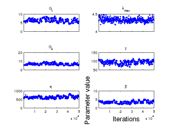
Chain Panel displays the burn-in rate of each parameter. If the parameter maintains a fixed distribution of values over the range of samples simulated, we can more confidently say that the posterior density has converged. In this particular example, this is not the case. The chains often "wander" suggesting multiple minima may be present or a lack of parameter sensitivity. Identification of both rate independent hyperelastic parameters and viscoelastic parameters is not easily determined from a single stretch rate. This suggest more data at different stretch rates should be used to more accurately quantify the distributions of the model parameters.

figure(3)
mcmcplot(chain,[],results.names,'chainpanel')
FSn = 18;
xlabel('Iterations', FS, FSn)
ylabel('Parameter value', FS, FSn)

% -------------------------------------------------------------------------
% Generate credible/prediction intervals using Bayesian Analysis
figure(4)
mcmcpredplot(out);
hold on
hd = plot(data.xdata, data.ydata,'b.', LW, 1, MS, 12);
hold off
grid on
FSn = 18;
xlabel('Stretch (\lambda) [-]', FS, FSn);
ylabel('Stress (\sigma) [kPa]', FS, FSn);
set(gca,FS,FSn);
ylim([0 250])
% Legend
legstr = {'95% CI', '95% PI', 'Model', 'Data'};
legh = legend(legstr);
set(legh, 'Orientation', 'Vertical', 'Location', 'NorthWest', FS, 15);
legend('boxoff');