clear all
Add MCMC codes to path
current_directory = cd;
addpath(strcat(current_directory,'/mcmcstat'));
The following analysis computes two electrostrictive parameters and a residual stress used in estimating changes in stress as a function of changes in the internal electronic state. The results are calculated from prior density functional theory (DFT) calculations. The DFT calculations were computed by incrementing atoms in lead titanate in a prescribed manner to produce changes in polarization about a fixed cubic strain state. This decouples the polarization energy and electrostriction for conducting independent energy and electrostrictive model calibration. More details about this analysis can be found in:
Oates, W., "A Quantum-informed Continuum Model for Ferroelectric Materials," Smart Mater. Struct. v. 23(10), p. 104009, 2014.
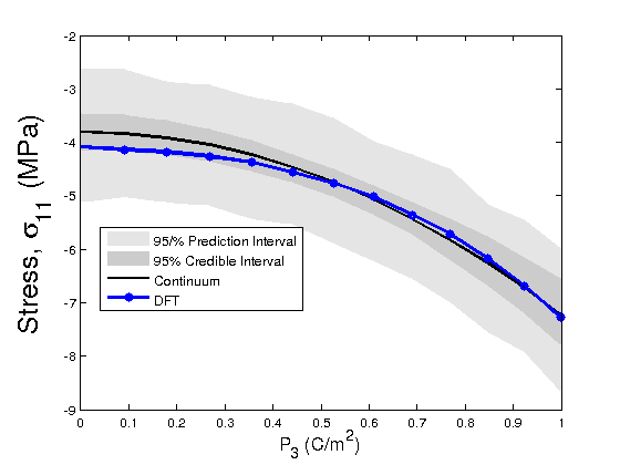
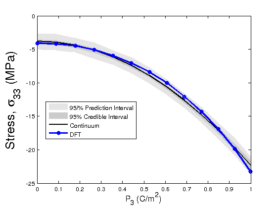
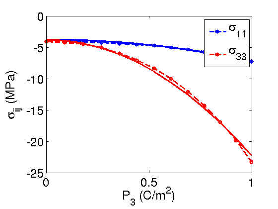
The form of the electrostrictive stress components considered for model calibration is
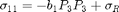
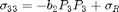
where  and
and  are the electrostrictive parameters and
  is the residual stress that will be calibrated through the Bayesian analysis. In this particular example, polarization
  in the
  direction is used which was calculated using the Berry phase approach in the DFT code ABINIT.
Define a function that calculates the sum of squares of error between the DFT stresses and the approximation based on the electrostrictive stress constitutive relation.
ssfun = @coupled_func_Bayesian;

model.ssfun = ssfun;
Load and apply variables for the DFT computational results for comparison to the electrostrictive constitutive law.
load DFT_cubic
model.N  = length(Pnum);

data.ydata_s11 = sig11_num;
data.ydata_s33 = sig33_num;
data.xdata = Pnum; %polarization computed from DFT using the Berry phase approach

%define initial guess for electrostrictive parameters
b1 = 3.4; %electrostrictive parameter
b2 = 18.5; %electrostrictive parameter
sigR = -3.8; %residual stress

tmin = [b1
        b2
        sigR];

%Electrostrictive model parameter range and initial guess
params = {
    {'b_1', tmin(1), -20, 20}
    {'b_2',  tmin(2), -20,50}
    {'\sigma^R',  tmin(3), -50,50}
    };
The next lines of code check the parameters prior to running a parameter estimation using MCMC.
[s11,s33] = coupled_model_Bayesian(tmin,data.xdata);
ss = coupled_func_Bayesian(tmin,data);
SS = ss/length(data.xdata);  %here is the cost calculation

figure(1)
axes1 = axes('FontSize',20);
plot((data.xdata),data.ydata_s11,'bo--','Linewidth',3)
hold on
plot((data.xdata),data.ydata_s33,'ro--','Linewidth',3)
plot((data.xdata),s11,'b-','Linewidth',3)
plot((data.xdata),s33,'r-','Linewidth',3)
hold off
ylabel('\sigma_{ij} (MPa)','FontSize',20)
xlabel('P_3 (C/m^2)','FontSize',20)
legend('\sigma_{11}','\sigma_{33}')
legend1 = legend(axes1,'show');
set(legend1,'EdgeColor',[1 1 1],'YColor',[1 1 1],'XColor',[1 1 1]);

variance = sum((data.ydata_s33-s33).^2)/(length(s33-1)); %estimation of the variance based on one
                                                         %stress component,
                                                         %s33

%
Bayesian MCMC Statistical analysis
model.S20 = variance/1e3; %estimate of variance based on prior simulation
model.N0  = 1;
model.N  = length(Pnum);
options.updatesigma=1;
options.method = 'dram';  %this applies the DRAM algorithm

options.nsimu = 1000; %run an initial small set of iterations prior to larger run
[results, chain, s2chain] = mcmcrun(model,data,params,options);

options.nsimu = 5000; %run longer simulations using results from smaller run as
                      %initial conditions
[results, chain, s2chain] = mcmcrun(model,data,params,options,results);
%
Setting nbatch to 1
Sampling these parameters:
name   start [min,max] N(mu,s^2)
b_1: 3.4 [-20,20] N(0,Inf)
b_2: 18.5 [-20,50] N(0,Inf)
\sigma^R: -3.8 [-50,50] N(0,Inf)
Setting nbatch to 1
Using values from the previous run
Sampling these parameters:
name   start [min,max] N(mu,s^2)
b_1: 3.61204 [-20,20] N(0,Inf)
b_2: 18.2685 [-20,50] N(0,Inf)
\sigma^R: -3.8265 [-50,50] N(0,Inf)
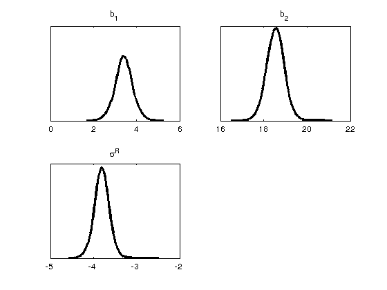
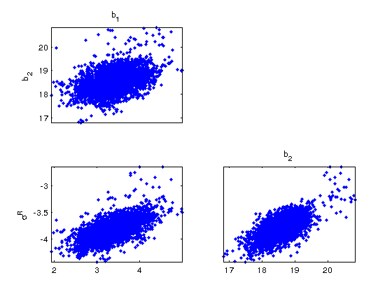
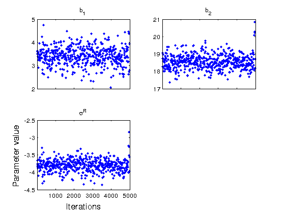
Plot results
figure(2)
mcmcplot(chain,[],results,'denspanel',2);
figure(3)
mcmcplot(chain,[],results,'pairs');

figure(4); clf
mcmcplot(chain,[],results.names,'chainpanel')
xlabel('Iterations','Fontsize',14)
ylabel('Parameter value','Fontsize',14)

chainstats(chain,results) %summary of parameter means, standard deviations, etc.
MCMC statistics, nsimu = 5000

                 mean         std      MC_err         tau      geweke
---------------------------------------------------------------------
       b_1     3.4099     0.39673    0.019018      9.8768      0.9796
       b_2     18.549     0.41905    0.023486      14.598     0.99524
  \sigma^R    -3.8048     0.17459    0.009535      11.974     0.99113
---------------------------------------------------------------------
Define a model function that calls the chains for error propagation. Plot the error propagation for both stress components  $ (s11) and
  $ (s33).
modelfun1 = @(d,th)coupled_model_predict_s11(th,d); %for stress component s11

%The following lines of code propagate the posterior densities of
%parameters to determine prediction and credible intervals of the Landau
%energy with respect to the DFT energy in light of the Bayesian statistics
nsample = 500;
out = mcmcpred(results,chain,s2chain,data.xdata,modelfun1,nsample);

figure(5)
modelout = mcmcpredplot(out); %,data
hold on
plot(data.xdata,data.ydata_s11,'bo-','linewidth',3)
hold off
xlabel('P_{3} (C/m^2)','Fontsize',14);
ylabel('Stress, \sigma_{11} (MPa)','FontSize',20)
legend('95/% Prediction Interval','95% Credible Interval','Continuum','DFT','Location','Best')

%Define a model function that calls the chains for error propagation
modelfun1 = @(d,th)coupled_model_predict_s33(th,d); %for stress component s_33

%The following lines of code propagate the posterior densities of
%parameters to determine prediction and credible intervals of the Landau
%energy with respect to the DFT energy in light of the Bayesian statistics
nsample = 500;
out = mcmcpred(results,chain,s2chain,data.xdata,modelfun1,nsample);

figure(6)
modelout = mcmcpredplot(out); %,data
hold on
plot(data.xdata,data.ydata_s33,'bo-','linewidth',3)
hold off
xlabel('P_{3} (C/m^2)','Fontsize',14);
ylabel('Stress, \sigma_{33} (MPa)','FontSize',20)
legend('95/% Prediction Interval','95% Credible Interval','Continuum','DFT','Location','Best')