clear all
The following lines of code add a path to all the Bayesian statistical functions.
% Add MCMC codes to path
current_directory = cd;
addpath(strcat(current_directory,'/mcmcstat'));
The following analysis computes two Landau energy parameters used in estimating changes in energy calculated from prior density functional theory (DFT) calculations. The DFT calculations were computed by incrementing atoms in lead titanate in a prescribed manner to produce changes in polarization about a fixed cubic strain state. Thus, only the polarization energy is required for model calibration. The effect of electrostriction is treated differently using a separate model for stress. More details about this analysis can be found in:
Oates, W., "A Quantum-informed Continuum Model for Ferroelectric Materials," Smart Mater. Struct. v. 23(10), p. 104009, 2014.
The form of the energy modeled considered for model calibration is
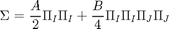
where  and
and  are the Landau parameters that will be calibrated through the Bayesian analysis. The vector order parameter is denoted by
  with
with  and is proportional to polarization.
Define a function that calculates the sum of squares of error between the DFT energy and the approximation based on the Landau continuum energy function.
ssfun = @coupled_func_Bayesian;

model.ssfun = ssfun;
Load the DFT calculations to fit the continuum scale Landau energy. A scaling parameter is introduced (1e3) that converts the energy from GPa units to MPa units. This scaling is applied on the initial parameter estimates and their bounds if the user wants to use a different set of units in fitting Landau energy parameters.
load DFT_cubic
model.N  = length(Pnum); %length of the different polarization and energy states

scaling = 1e3; %all DFT energy density is in units of MPa using the scaling 1e3

%cubic volume
V0 = 4.1476034E+02; %volume of DFT lattice in Bohr^3
V1 = V0*(5.29177249e-11)^3; %conversion of volume to m^3
deltaE = (E_tot - E_tot(1))/V1*1.60217656535e-19/1e9; %Giga-Joules/m^3 conversion from eV/m^3

%input energy paramters from DFT
data.ydata_E_tot = deltaE*scaling;
data.xdata = Pnum; %polarization computed from DFT using the Berry phase approach

%define initial guess for Landau parameters
A = -0.805*scaling;
B = 3.32*scaling;
tmin = [A
        B];

%Landau energy model parameter range and initial guess
params = {
    {'A', tmin(1), -5e6*scaling, 5e6*scaling}
    {'B',  tmin(2), -5e3*scaling,5e8*scaling}
    };
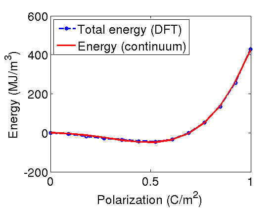
Check model initial output prior to running a parameter estimation using MCMC
[Sigma] = coupled_model_Bayesian(tmin,data.xdata);
ss = coupled_func_Bayesian(tmin,data);
SS = ss/length(data.xdata);  %here is the cost calculation

figure(1)
axes1 = axes('FontSize',20);
plot(Pnum,data.ydata_E_tot,'bo--','Linewidth',3)
hold on
plot(Pnum,Sigma,'r-','Linewidth',3)
hold off
ylabel('Energy (MJ/m^3)','FontSize',20)
xlabel('Polarization (C/m^2)','FontSize',20)
legend('Total energy (DFT)','Energy (continuum)','Location','NorthWest')
legend1 = legend(axes1,'show');
set(legend1,'EdgeColor',[1 1 1],'YColor',[1 1 1],'XColor',[1 1 1]);

variance = sum((data.ydata_E_tot-Sigma').^2)/(length(deltaE-1)); %calculate the variance
Run the Bayesian statistical analysis. An initial run with a smaller number of iterations is first done and used as initial results in a longer set of iterations.
model.S20 = variance;%estimate of variance based on prior simulation
model.N0  = 1;
model.N  = length(Pnum);
options.updatesigma=1;
options.method = 'dram';  %this applies the DRAM algorithm

options.nsimu = 500; %run an initial small set of iterations prior to larger run
[results, chain, s2chain] = mcmcrun(model,data,params,options);

options.nsimu = 10000; %run longer simulations using results from smaller run as
                      %initial conditions
[results, chain, s2chain] = mcmcrun(model,data,params,options,results);
Setting nbatch to 1
Sampling these parameters:
name   start [min,max] N(mu,s^2)
A: -805 [-5e+09,5e+09] N(0,Inf)
B: 3320 [-5e+06,5e+11] N(0,Inf)
Setting nbatch to 1
Using values from the previous run
Sampling these parameters:
name   start [min,max] N(mu,s^2)
A: -787.005 [-5e+09,5e+09] N(0,Inf)
B: 3272.77 [-5e+06,5e+11] N(0,Inf)
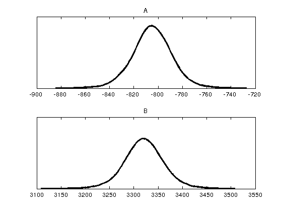
Plot results.
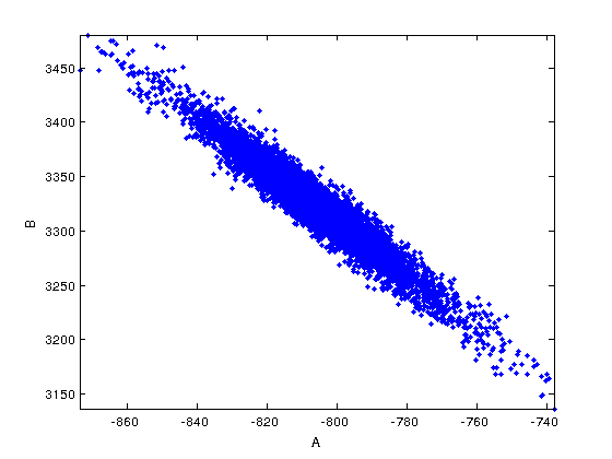
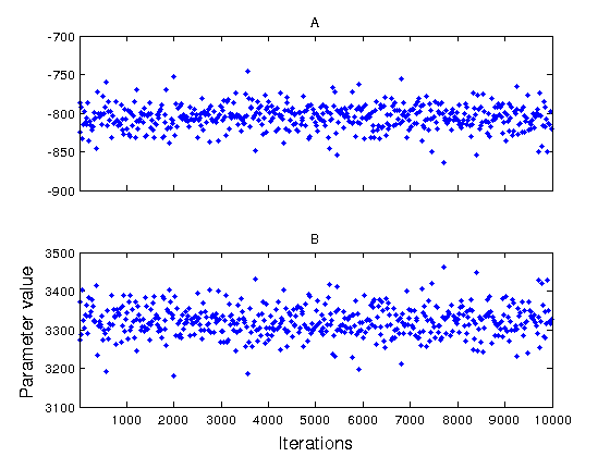
figure(2)
mcmcplot(chain,[],results,'denspanel',2);
figure(3)
mcmcplot(chain,[],results,'pairs');

figure(4); clf
mcmcplot(chain,[],results.names,'chainpanel')
xlabel('Iterations','Fontsize',14)
ylabel('Parameter value','Fontsize',14)

chainstats(chain,results) %summary of parameter means, standard deviations, etc.
MCMC statistics, nsimu = 10000

                 mean         std      MC_err         tau      geweke
---------------------------------------------------------------------
         A    -804.99      16.144      0.5056      6.9381     0.99921
         B     3320.7      40.049      1.1616       6.974     0.99928
---------------------------------------------------------------------
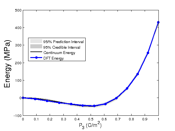
Define a model function that calls the chains for error propagation that give calculation of prediction and credible intervals
modelfun1 = @(d,th)coupled_model_Bayesian(th,d); % NOTE: the order in which d and th appear is important

%The following lines of code propagate the posterior densities of
%parameters to determine prediction and credible intervals of the Landau
%energy with respect to the DFT energy in light of the Bayesian statistics
nsample = 500;
out = mcmcpred(results,chain,s2chain,data.xdata,modelfun1,nsample);

figure(5)
modelout = mcmcpredplot(out); %,data
hold on
plot(data.xdata,data.ydata_E_tot,'bo-','linewidth',3)
hold off
xlabel('P_{3} (C/m^2)','Fontsize',14);
ylabel('Energy (MPa)','FontSize',20)
legend('95/% Prediction Interval','95% Credible Interval','Continuum Energy','DFT Energy','Location','Best')