Pipes are all around us. Every time we turn the faucet, we expect water to come out. We expect there to be sufficient pressure to get the job done, be it filling a glass of water in a timely manner or taking a nice shower. A lot of experimentation went behind the selection of pipe sizes used in various applications to ensure that what comes out is acceptable.
In the plumbing industry there are rules of thumb for sizing pipes for a given use. This is usually a matter of picking the right pipe diameter for the use. For example, you wouldn't use 2 inch diameter PVC pipe to run water to a bathroom sink. Nor would you use 1/8 inch pipes for a drain for the same sink. The pipe flow experiment provides an experimental backbone or learning how to apply engineering equations to real world situations where fluids flow.
Experiment 100: Pipe Flow involves an experimental apparatus with:
Some things that can be done with this apparatus:
This experiment is relatively simple. Reguardless of this fact, all the required Personal Protective Equipment should be worn by all team members while in the lab. Two devices used, one manometer and one thermometer, contain mercury. The mercury used in the mercury manometer should be watched carefully to insure that the mercury does not come out of the manometer. When measuring the temperature of the reservoir, the thermometer should be carefully handled to insure that the mercury is not spilled, which would happen if the glass were broken. As with any hazardous material, all team members working on or near this apparatus should be fully aware of what they are near. With this in mind, all team members should read and understand the Materials Safety Data Sheet for mercury before entering the lab.
Though water is not a hazardous material, it can cause an accident when it is spilled on the floor. The water should be quickly mopped up with the mop to reduce the chances of an accident. The pressure taps and tubing can cause accidents to occur because of their lengths and bulky masses. Make sure they are properly stored when they are not in use.
The flow of a fluid through a pipe is governed by various equations, representing the array of factors that control flow conditions. Bernoulli's Equation relates the pressure loss in the pipe to a change in the average fluid velocity. That equation is the fundamental equation for understanding general pipe flow. The Reynolds number describes which flow regime is present in piping. It describes the relationship that exists between the fluid's velocity and the density. The Fanning Friction Factor relates the shear stress to the average kinetic energy of the fluid. Pipe diameter and length also are mitigating factors in this equation.
The basic approach to all piping systems is to write the Bernoulli equation between two points, connected by a streamline, where the conditions are known.
Dv2/2 + gDz + DP/r + Ws + F = 0
The average velocity is the ratio between the volumetric flow rate and the cross-sectional area of the pipe.
Vave = Q/A
The frictional dissipation can be used to describe the friction loss in the pipe. Mathematically, the definition is:
We calculate the Reynolds number so that we can easily tell if the flow is in the laminar or turbulent regime.
Re = (vave* Dpipe)/ n
Laminar regime 2100 < Re
![]() 4000
4000
Turbulent regime Re > 4000
A good example of laminar and turbulent flow is the rising smoke from a cigarette. The smoke initially travels in smooth, straight lines (laminar flow) then starts to randomly mix (turbulent flow). These ranges are discussed above.
|
Symbol |
Description |
|
Re, dimensionless |
Reynolds Number |
|
r, kg/m3 |
Density |
|
vave, m/s |
Average Velocity |
|
v, m2/s |
Kinematic Viscosity |
|
D, m |
Diameter |
|
Q, m3/s |
Volumetric flow rate |
|
A, m2 |
Cross sectional area |
|
Ws, J |
Shaft Work |
|
ffexp, dimensionless |
Experimental Frictional Dissipation |
|
DP, kg/(m*s2) |
Change in Pressure |
|
g, m/s2 |
Gravity |
|
L, m |
Length |
In this experiment, water flowing through varying diameter pipes is observed. The resulting pressure drops from changing the water velocity are used to calculate the Reynolds number, the water velocity, and friction factor.
Several friction factor equations are available for systems of flow depending on the type of flow present (laminar or turbulent) and the interior surfaces through which the flow takes place. Using the equations for friction factor in laminar and/or turbulent flow, the friction factor can be determined. In order to find the friction factor we first have to determine the Reynolds number. This is done for water by obtaining waters density and viscosity at the operating temperatures, the interior diameter of the pipe, and the roughness coefficient of the pipe. An empirical equation is then used to compare the experimental results to theoretical results.
Using the equations for friction factor in laminar and/or turbulent flow, a correlation between Reynolds number and friction factor can be found. The friction factor in all cases depends upon the Reynolds number. For laminar flow the correlation gives a steeper slope than for turbulent flow. The relationship seen between the friction factor and the Reynolds number for turbulent suggest that at large flow rates the friction factor becomes less dependent on the Reynolds number.
Using the equation for calculating volumetric flow rate, the mean velocity can be calculated knowing the area of the pipe. The velocity of the smallest pipe can be found by the volumetric flow rate, which is found by measuring the time it takes for the water to fill a container with a known volume. An orifice meter along with the appropriate orifice equation will also be used to determine the volumetric flow rate. That flow rate will then be converted to a velocity.
The radius, r, is the radial position from the axis of the pipe and the radius, R, is the radius of the pipe. The velocity, v, is the velocity in the pipe and the velocity, vmax, is the maximum velocity in the pipe. The velocity varies as a function of the radial position in the pipe. At the maximum radius, the velocity will be zero while at the very center of the pipe; the velocity will be at its maximum. The pitot tube will be used to measure how the velocity varies with the radius on the large tube. By adjusting the Pitot tube to cover its full radial range and by using water manometer applications, we can calculate experimental volumetric flow rates. Using the appropriate equations, this flow rate can be manipulated to find the velocity at certain radial positions within the pipe.
The velocity and pressure drop in turbulent flow is measured in this experiment. These values will then be compared to the Hagen-Poiseuille relationship for laminar flow. This objective can be better completed outside of the laboratory using library references and sources. Once the comparison between the Hagen-Poiseuille relationship and the turbulent flow regime has been made, it can be applied to our experimental results to check for correlations and/or shortcomings.
These links take you off this site.
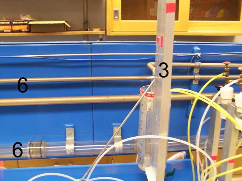
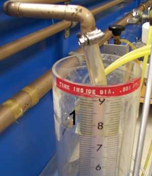
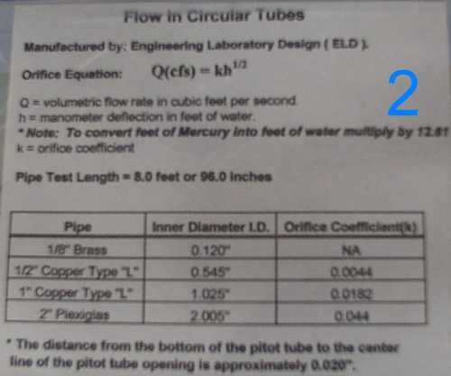
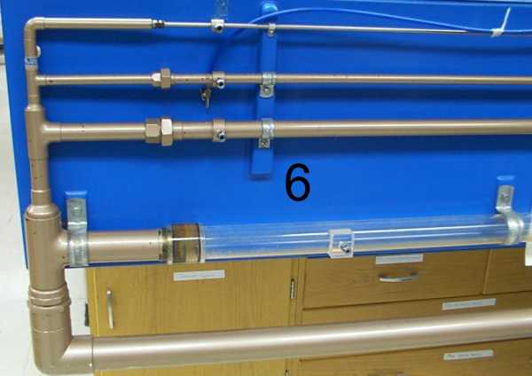
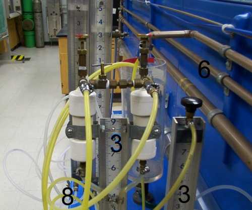
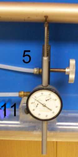
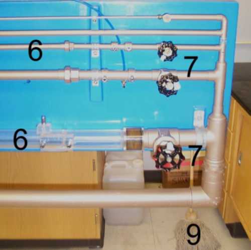
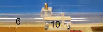
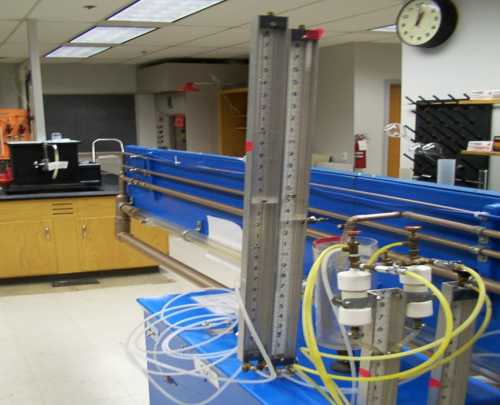
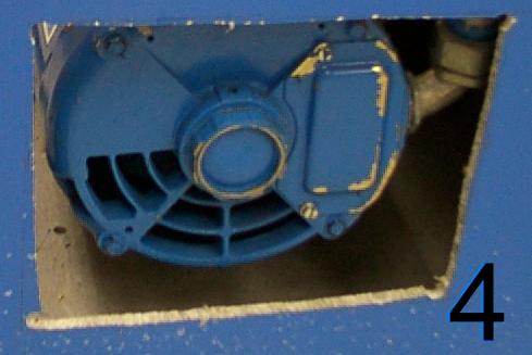
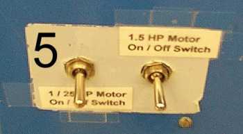
The following figures are digital images taken of the pipe flow apparatus used in this experiment.
| Number | Description |
| 1 | Volume container for smallest diameter pipe |
| 2 | Diameters and orifice equation for Pipes |
| 3 | Manometers |
| 4 | Water Pump |
| 5 | Water Pump On/Off Switches |
| 6 | Pipes |
| 7 | Pipe Valves |
| 8 | Plastic Tubing |
| 9 | Mop |
| 10 | Pressure Taps |
| 11 | Pitot Tube |
|
|
|
|
|
This document was generated using the LaTeX2HTML translator Version 2K.1beta (1.48)
Copyright © 1993, 1994, 1995, 1996,
Nikos Drakos,
Computer Based Learning Unit, University of Leeds.
Copyright © 1997, 1998, 1999,
Ross Moore,
Mathematics Department, Macquarie University, Sydney.
The command line arguments were:
latex2html -split 0 -show_section_numbers /tmp/lyx_tmpdir3481JKjPT4/lyx_tmpbuf3481zZG8JY/exp100-03web3274l.tex
The translation was initiated by root on 2001-10-14