|
|
|
|
|
Next: A.16 The adiabatic theorem |
|
The classical
quantum theory discussed in this book
runs into major difficulties with truly relativistic effects. In
particular, relativity allows particles to be created or destroyed.
For example, a very energetic photon near a heavy nucleus might create
an electron and a positron. Einstein’s ![]()
![]()
![]()
quantum field theory
is needed.
And quantum field theory is not just for esoteric conditions like
electron-positron pair creation. The photons of light are routinely
created and destroyed under normal conditions. Still more basic to an
engineer, so are their equivalents in solids, the phonons of crystal
vibrations. Then there is the band theory of semiconductors:
electrons are created
within the conduction band, if
they pick up enough energy, or annihilated
when they
lose it. And the same happens for the real-life equivalent of
positrons, holes in the valence band.
Such phenomena are routinely described within the framework of quantum field theory. Almost unavoidably you will run into it in literature, [18,29]. Electron-phonon interactions are particularly important for engineering applications, leading to electrical resistance (along with crystal defects and impurities), and to the combination of electrons into Cooper pairs that act as bosons and so give rise to superconductivity.
This addendum explains some of the basic ideas of quantum field theory. It should allow you to recognize it when you see it. Addendum {A.23} uses the ideas to explain the quantization of the electromagnetic field. That then allows the quantum description of spontaneous emission of radiation by excited atoms or nuclei in {A.24}. Here a photon is created.
Unfortunately a full discussion of quantum field theory is far outside the scope of this book. Especially the fully relativistic theory is very involved. To explain quantum field theory in a nutshell takes Zee 500 pages, [53]. Tong [[17]] writes: “This is charming book, where emphasis is placed on physical understanding and the author isn’t afraid to hide the ugly truth when necessary. It contains many gems.” But you first need to learn linear algebra, at the minimum read all of chapter 1 on relativity, chapter 1.2.5 and {A.4} on index notation, chapter 12.12 and {A.36} on the Dirac equation, addendum {A.14} on the Klein-Gordon equation, {A.1} on Lagrangian mechanics, {A.12} on the Heisenberg interpretation, and pick up enough group theory. Learning something about the path integral approach to quantum mechanics, like from [22], cannot hurt either. In the absence of 1 000 pages and a willing author, the following discussion will truly be quantum field theory in a nanoshell.
If you want to get a start on a more advanced treatment of quantum field theory of elementary particles at a relatively low level of mathematics, Griffiths [24] is recommended.
And if you are just interested in relativistic quantum mechanics from an intellectual point of view, there is good news. Feynman gave a set of lectures on “quantum electrodynamics” for a general audience around 1983, and the text is readily available at low cost. Without doubt, this is the best exposition of the fundamentals of quantum mechanics that has ever been written, or ever will. The subject is reduced to its bare abstract axioms, and no more can be said. If the human race is still around a millennium or so from now, artificial intelligence may take care of the needed details of quantum mechanics. But those who need or want to understand what it means will still reach for Feynman. The 2006 edition, [19], has a foreword by Zee that gives a few hints how to relate the basic concepts in the discussion to more conventional mathematics like the complex numbers found in this book. It will not be much help applying quantum field theory to engineering problems, however.
The first concept that must be understood in quantum field theory is occupation numbers. They will be the new way to represent quantum wave functions.
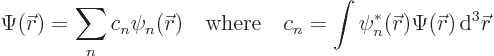
Recall first the form of wave functions in classical
quantum mechanics, as normally covered in this book. Assume a system
of independent, or maybe weakly interacting particles. The energy
eigenfunctions of such a system can be written in terms of whatever
are the single-particle energy eigenfunctions
Now consider a system of, say, 36 particles. A completely arbitrary
example of an energy eigenfunction for such a system would be:
 |
Instead of writing out the example eigenfunction mathematically as
done in (A.46) above, it can be graphically depicted as in
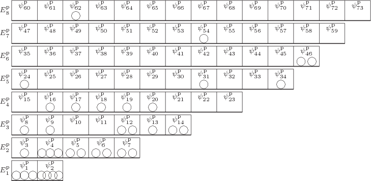
figure A.2. In the figure the single-particle states
are shown as boxes, and the particles that are in those particular
single-particle states are shown inside the boxes. In the example,
particle 1 is inside the ![]()
![]()
 |
However, if the 36 particles are identical bosons, (like photons or
phonons), the example mathematical eigenfunction (A.46) and
corresponding depiction figure A.2 is unacceptable. As
chapter 5.7 explained, wave functions for bosons must be
unchanged if two particles are swapped. But if, for example,
particles 2 and 5 in eigenfunction (A.46) above are
exchanged, it puts 2 in state 6 and 5 in state 4:

It is much easier in terms of the graphical depiction figure A.2: graphically all these countless system eigenfunctions differ only with respect to the numbers in the particles. And since in the final eigenfunction, all particles are present in exactly the same way, then so are their numbers within the particles. Every number appears equally in every particle. So the numbers do no longer add distinguishing information and can be left out. That makes the graphical depiction of the example eigenfunction for a system of identical bosons as in figure A.3. It illustrates why identical particles are commonly called “indistinguishable.”
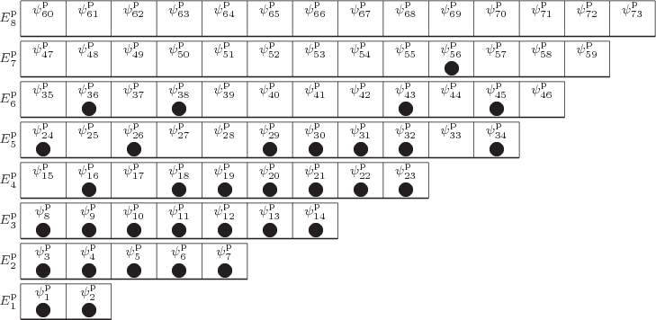 |
For a system of identical fermions, (like electrons or quarks), the
eigenfunctions must change sign if two particles are swapped. As
chapter 5.7 showed, that is very restrictive. It means
that you cannot create an eigenfunction for a system of 36 fermions
from the example eigenfunction (A.46) and the swapped
versions of it. Various single-particle eigenfunctions appear
multiple times in (A.46), like ![]() ,
,
It is the same graphically. The example figure A.3 for bosons is impossible for a system of identical fermions; there cannot be more than one fermion in a single-particle state. A depiction of an arbitrary energy eigenfunction that is acceptable for a system of 33 identical fermions is in figure A.4.
As explained in chapter 5.7, a neat way of writing down
the system energy eigenfunction of the pictured example is to form a
Slater determinant from the occupied states
Now consider what happens in relativistic quantum mechanics. For
example, suppose that an electron and positron annihilate each other.
What are you going to do, leave holes in the parameter list of your
wave function, where the electron and positron used to be? Like
And if positrons are too weird for you, consider photons, the particles of electromagnetic radiation, like ordinary light. As chapters 6.8 and 7.8 showed, the electrons in hot surfaces create and destroy photons readily when the thermal equilibrium shifts. Moving at the speed of light, with zero rest mass, photons are as relativistic as they come. Good luck scribbling in trillions of new states for the photons into your wave function when your black box heats up. Then there are solids; as chapter 11.14.6 shows, the phonons of crystal vibrational waves are the equivalent of the photons of electromagnetic waves.
One of the key insights of quantum field theory is to do away with classical mathematical forms of the wave function such as (A.46) and the Slater determinants. Instead, the graphical depictions, such as the examples in figures A.3 and A.4, are captured in terms of mathematics. How do you do that? By listing how many particles are in each type of single-particle state. In other words, you do it by listing the single-state “occupation numbers.”
Consider the example bosonic eigenfunction of figure
A.3. The occupation numbers for that state would be
General wave functions can be described by taking linear combinations
of these basis states. The most general Fock wave function for a
classical set of exactly ![]()
![]() .
.Fock space.
How about the case of distinguishable particles as in figure A.2? In that case, the numbers inside the particles also make a difference, so where do they go?? The answer of quantum field theory is to deny the existence of generic particles that take numbers. There are no generic particles in quantum field theory. There is a field of electrons, there is a field of protons, (or quarks, actually), there is a field of photons, etcetera, and each of these fields is granted its own set of occupation numbers. There is no way to describe a generic particle using a number. For example, if there is an electron in a single-particle state, in quantum field theory it means that the electron field has a particle in that energy state. The particle has no number.
Some physicist feel that this is a strong point in favor of believing that quantum field theory is the way nature really works. In the classical formulation of quantum mechanics, the (anti) symmetrization requirements under particle exchange are an additional ingredient, added to explain the data. In quantum field theory, it comes naturally: particles that are distinguishable simply cannot be described by the formalism. Still, our convenience in describing it is an uncertain motivator for nature.
The successful analysis of the blackbody spectrum in chapter 6.8 already testified to the usefulness of the Fock space. If you check the derivations in chapter 11 leading to it, they were all conducted based on occupation numbers. A classical wave function for the system of photons was never written down; that simply cannot be done.
There is a lot more involved in quantum field theory than just the
blackbody spectrum, of course. To explain some of the basic ideas,
simple examples can be helpful. The simplest example that can be
studied involves just one single-particle state, say just a
single-particle ground state. The graphical depiction of an arbitrary
example wave function is then as in figure A.5. There is
just one single-particle box. In nonrelativistic quantum mechanics,
this would be a completely trivial quantum system. In the case of ![]()
But when particles can be created or destroyed, things get more
interesting. When there is no given number of particles, there can be
any number of identical bosons within that single particle state.
That allows ![]()
![]()
![]()
![]()
![]()
A relativistic system with just one type of single-particle state does seem very artificial. It raises the question how esoteric such an example is. But there are in fact two very well established classical systems that behave just like this:
particlesto be quanta of energy of size
Recall from chapter 4.1 that there is an additional
ground state energy of half a ![]()
vacuum energy.
The general wave function of a harmonic oscillator is a linear combination of the energy states. In terms of chapter 4.1, that expresses an uncertainty in energy. In the present context, it expresses an uncertainty in the number of these energy particles!
particlesto be single quanta of
particleand the state with no angular momentum
particle.
This example is less intuitive, since normally when you talk about a particle, you talk about an amount of energy, like in Einstein’s mass-energy relation. If it bothers you, think of the electron as being confined inside a magnetic field; then the spin-up state is associated with a corresponding increase in energy.
relativisticsystems with only one single-particle state are obviously made up, they do provide a very valuable sanity check on any relativistic analysis.
Not only that, the two examples are also very useful to understand the
difference between a zero wave function and the so-called “vacuum state”
Fock basis kets are taken to be orthonormal; an inner product between
kets is zero unless all occupation numbers are equal. If they are all
equal, the inner product is 1. In short:
If the two kets have the same total number of particles, this orthonormality is required because the corresponding classical wave functions are orthonormal. Inner products between classical eigenfunctions that have even a single particle in a different state are zero. That is easily verified if the wave functions are simple products of single-particle ones. But then it also holds for sums of such eigenfunctions, as you have for bosons and fermions.
If the two kets have different total numbers of particles, the inner
product between the classical wave functions does not exist. But
basis kets are still orthonormal. To see that, take the two simple
examples given above. For the harmonic oscillator example, different
occupation numbers for the particles
correspond to
different energy eigenfunctions of the actual harmonic oscillator.
These are orthonormal. It is similar for the spin example. The state
of 0 particles
is the spin-down state of the electron.
The state of 1 particle
is the spin-up state. These
spin states are orthonormal states of the actual electron.
The key to relativistic quantum mechanics is that particles can be
created and annihilated. So it may not be surprising that it is very
helpful to define operators that create
and
annihilate
particles .
To keep the notations relatively simple, it will initially be assumed that there is just one type of single-particle state. Graphically that means that there is just one single-particle state box, like in figure A.5. However, there can be an arbitrary number of particles in that box.
The desired actions of the creation and annihilation operators are
sketched in figure A.6. An annihilation operator ![]()
![]()
![]()
![]()
![]()
![]()
![]()
![]()
![]()
![]()
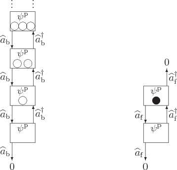 |
The operators are therefore defined by the relations
Note that the above relations only specify what the operators ![]()
![]()
Mathematically you can always define whatever operators you want. But
you must hope that they will turn out to be operators that are
physically helpful. To help achieve that, you want to chose the
numerical constants ![]()
![]()
If the constants ![]()
![]()
![]()
![]() ,
,![]()
The full definition of the annihilation and creation operators can now
be written in a nice symmetric way as
These operators are particularly convenient since they are Hermitian
conjugates. That means that if you take them to the other side in an
inner product, they turn into each other. In particular, for inner
products between basis kets,
To verify that the above relations apply, recall from the previous
subsection that kets are orthonormal. In the equalities above, the
inner products are only nonzero if ![]()
![]()
![]() :
:![]() ,
,![]() ,
,![]()
![]()
![]() ,
,![]()
![]()
![]() ,
,
It remains true for fermions that ![]()
![]()
![]()
![]()
![]() .
.![]()
The inner products are usually written in the more esthetic form
You may well wonder why ![]()
![]() ?
?![]()
![]()
![]()
![]()
![]() .
.
Still, it is interesting to see what the effect of ![]()
The same commutator does not apply to fermions, because if you apply
![]()
![]() ,
,![]() .
.![]()
![]()
![]()
![]()
![]()
![]()
![]()
![]()
![]()
![]()
![]()
![]() ;
;
How about the Hamiltonian for the energy of the system of particles?
Well, for noninteracting particles the energy of ![]()
![]()
![]() .
.![]() ,
,![]() .
.
It is important to note that the creation and annihilation operators
![]()
![]()
![]()
![]()
Hermitian operators can also be formed from linear combinations of the
creation and annihilation operators. Two combinations that are often
physically relevant are
Conversely, the annihilation and creation operators can be written in
terms of the caHermitians as
The Hamiltonian (A.53) for noninteracting particles can be
written in terms of ![]()
![]()
What this Hamiltonian means depends on whether the particles being
described are bosons or fermions. They have different commutators
![]() .
.
Consider first the case that the particles are bosons. The previous
subsection showed that the commutator ![]()
![]()
![]()
The Hamiltonian for bosons becomes, using the commutator above,
For fermions, the following useful relations follow from the
anticommutators for the creation and annihilation operators given in
the previous subsection:
The arguments of the previous subsection can be reversed. Given a suitable Hamiltonian, it can be recast in terms of annihilation and creation operators. This is often useful. It provides a way to quantize systems such as a harmonic oscillator or electromagnetic radiation.
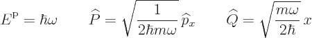
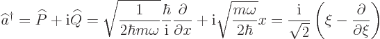
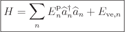
Assume that some system has a Hamiltonian with the following
properties:
![\begin{displaymath}
\fbox{$\displaystyle
H = {\vphantom' E}^{\rm p}\left(\wide...
...at P,\widehat Q\right] = - {\textstyle\frac{1}{2}} {\rm i}
$}
\end{displaymath}](img3985.gif) |
(A.59) |
It may be noted that typically ![]()
![]()
![]() ,
,![]() .
.![]()
![]() .
.
From the given apparently limited amount of information, all of the following conclusions follow:
amplitude
quantaof energy
The derivation of the above properties is really quite simple and elegant. It can be found in {D.33}.
Note that various properties above are exactly the same as found in the analysis of bosons starting with the annihilation and creation operators. The difference in this subsection is that the starting point was a Hamiltonian in terms of two square Hermitian operators; and those merely needed to have a purely imaginary commutator.
This subsection will illustrate the power of the introduced quantum field ideas by example. The objective is to use these ideas to rederive the one-dimensional harmonic oscillator from scratch. The derivation will be much cleaner than the elaborate algebraic derivation of chapter 4.1, and in particular {D.12}.
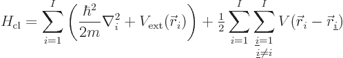
The Hamiltonian of a harmonic oscillator in classical quantum
mechanics is, chapter 4.1,
According to the previous subsection, a system like this can be solved
immediately if the commutator of ![]()
![]()
To use the results of the previous subsection, first the Hamiltonian
must be rewritten in the form
According to the previous subsection, the energy eigenvalues are
And various other interesting properties of the solution may also be found in the previous subsection. Like the fact that there is half a quantum of energy left in the ground state. True, the zero level of energy is not important for the dynamics. But this half quantum does have a physical meaning. Assume that you have a lot of identical harmonic oscillators in the ground state, and that you do a measurement of the kinetic energy for each. You will not get zero kinetic energy. In fact, the average kinetic energy measured will be a quarter quantum, half of the total energy. The other quarter quantum is what you get on average if you do potential energy measurements.
Another observation of the previous subsection is that the expectation position of the particle will vary harmonically with time. It is a harmonic oscillator, after all.
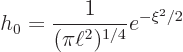
The energy eigenfunctions will be indicated by ![]() ,
,![]() .
.![]()
![]() ,
,
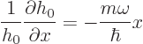
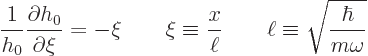
Integrating both sides with respect to ![]()
!in the notations section. That gives the final ground state as
To get the other eigenfunctions ![]()
![]()
![]()
![]()
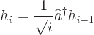
That was easy, wasn’t it?
“Canonical quantization” is a procedure to turn a classical system into the proper quantum one. If it is applied to a field, like the electromagnetic field, it is often called “second quantization.”
Recall the quantum analysis of the harmonic oscillator in the previous subsection. The key to the correct solution was the canonical commutator between position and momentum. Apparently, if you get the commutators right in quantum mechanics, you get the quantum mechanics right. That is the idea behind canonical quantization.
The basic idea can easily be illustrated for the harmonic oscillator.
The standard harmonic oscillator in classical physics is a simple
spring-mass system. The classical governing equations are:
As you can readily check by substitution, the most general solution is

amplitude
frequency
This system is now to be quantized using canonical quantization. The
process is somewhat round-about. First a “canonical momentum,” or “conjugate momentum,” or “generalized momentum,” ![]()
![]() ,
,![]() .
.![]()
![]() ,
,![]() .
.
Next a classical Hamiltonian is defined. It is the total energy of
the system expressed in terms of position and momentum:
To quantize the system, the momentum and position in the Hamiltonian
must be turned into operators. Actual values of momentum and position
are then the eigenvalues of these operators. Basically, you just put
a hat on the momentum and position in the Hamiltonian:
In general, you identify commutators in quantum mechanics with
so-called Poisson brackets
in classical mechanics.
Assume that ![]()
![]()
![]()
![]() .
.
Because of reasons discussed for the Heisenberg picture of quantum mechanics, {A.12}, the procedure ensures that the quantum mechanics is consistent with the classical mechanics. And indeed, the results of the previous subsection confirmed that. You can check that the expectation position and momentum had the correct classical harmonic dependence on time.
Fundamentally, quantization of a classical system is just an educated guess. Classical mechanics is a special case of quantum mechanics, but quantum mechanics is not a special case of classical mechanics. For the material covered in this book, there are simpler ways to make an educated guess than canonical quantization. Being less mathematical, they are more understandable and intuitive. That might make them maybe more convincing too.
There is, of course, not much analysis that can be done with a fermion system with only one single-particle state. There are only two independent system states; no fermion or one fermion.
However, there is at least one physical example of such a simple
system. As noted in subsection A.15.1, a particle with
spin ![]()
![]()
![]()
![]()
![]() -
-
One reasonable question that can now be asked is whether the annihilation and creation operators, and the caHermitians, have some physical meaning for this system. They do.
Recall that for fermions, the Hamiltonian was given in terms of the
caHermitians ![]()
![]()
![\begin{displaymath}[\widehat P_{\rm {f}},\widehat Q_{\rm {f}}]= {\rm i}\frac{{\widehat S}_z}{\hbar}
\end{displaymath}](img4032.gif)
Reasonably speaking then, the caHermitians themselves should be the
nondimensional components of spin in the ![]()
![]()
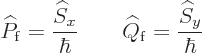
Recall another property of the caHermitians for fermions:
Finally consider the annihilation and creation operators, multiplied
by ![]() :
:
Obviously, you can learn a lot by taking a quantum field type
approach. To be sure, the current analysis applies only to particles
with spin ![]() .
.
The previous subsections discussed quantum field theory when there is
just one type of single-particle state for the particles. This
subsection considers the case that there is more than one. An index
![]()
Graphically, the case of multiple single-particle states was
illustrated in figures A.3 and A.4.
There is now more than one box that particles can be in. Each box
corresponds to one type of single-particle state ![]() .
.
Each such single-particle state has an occupation number ![]()
An annihilation operator ![]()
![]()
The commutator relations are
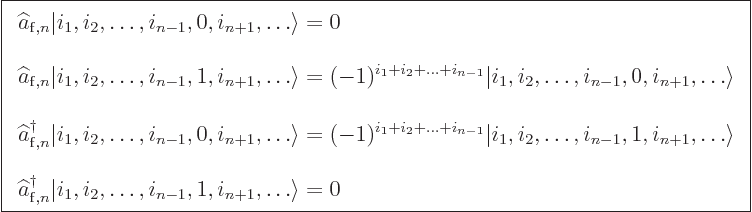
For fermions it is a bit more complex. The graphical representation
of the example fermionic energy eigenfunction figure
A.4 cheats a bit, because it suggests that there is
only one classical wave function for a given set of occupation
numbers. Actually, there are two variations, based on how the
particles are ordered. The two are the same except that they have the
opposite sign. Suppose that you create a particle in a state
![]() ;
;![]() ,
,![]()
![]() .
.
What you can do is define the annihilation and creation operators for
fermions as follows:
Of course, you can define the annihilation and creation
operators with whatever sign you want, but putting in the sign pattern
above may produce easier mathematics. In fact, there is an immediate
benefit already for the anticommutator relations; they take the same
form as for bosons, except with anticommutators instead of
commutators:
The Hamiltonian for a system of noninteracting particles is like the
one for just one single-particle state, except that you must now sum
over all single-particle states:
As noted at the start of this section, quantum field theory is particularly suited for relativistic applications because the number of particles can vary. However, in relativistic applications, it is often necessary to work in terms of position coordinates instead of single-particle energy eigenfunctions. To be sure, practical quantum field computations are usually worked out in terms of relativistic energy-momentum states. But to understand them requires consideration of position and time. Relativistic applications must make sure that coordinate systems moving at different speeds are physically equivalent and related through the Lorentz transformation. There is also the “causality problem,” that an event at one location and time may not affect an event at another location and time that is not reachable with the speed of light. These conditions are posed in terms of position and time.
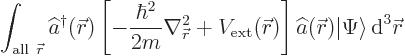
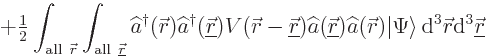
To handle such problems, the annihilation and creation operators can
be converted into so-called field operators
![]()
![]()
![]()
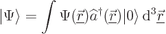
Now in classical quantum mechanics, a particle at a given position
![]()
![]() ,
,![]()
![]()
![]() ,
,![]()
![]()
![]()
![]() ,
,![]()
![]()
![]()
Like any function, a delta function can be written in terms of the
single-particle energy eigenfunctions ![]()
Since ![]()
![]()
![]() ,
,
| (A.65) |
In the case of noninteracting particles in free space, the energy
eigenfunctions are the momentum eigenfunctions
![]() .
.![]()
![]()
![]()
![]()
![]()
To check the appropriateness of the creation field operator as defined
above, consider its consistency with classical quantum mechanics. A
classical wave function ![]()
Now this needs to be converted to quantum field form. The classical
wave function then becomes a combination ![]()
![]()
![]()
![]() .
.
As a check on the appropriateness of the annihilation field operator,
consider the Hamiltonian. The Hamiltonian of noninteracting particles
satisfies
In terms of annihilation and creation field operators, you would like
the Hamiltonian to be defined similarly:
Now, if the definitions of the field operators are right, this
Hamiltonian should still produce the same answer as before.
Substituting in the definitions of the field operators gives
The above argument roughly follows [43, pp. 22-29], but
note that this source puts a tilde on ![]()
![]()
One final question that is much more messy is in what sense these
operators really create or annihilate a particle localized at
![]() .
.![]() .
.![]() .
.
A big advantage of the way the annihilation and creation operators
were defined now shows up: the annihilation and creation field
operators satisfy essentially the same (anti)commutation relations.
In particular
To check these commutators, plug in the definitions of the field
operators. Then the zero commutators above follow immediately from the
ones for ![]()
![]() ,
,![]()
![]() .
.![]() ,
,![]() .
.![]()
![]()
![]()
Field operators help solve a vexing problem for relativistic quantum mechanics: how to put space and time on equal footing, [43, p. 7ff]. Relativity unavoidably mixes up position and time. But classical quantum mechanics, as covered in this book, needs to keep them rigidly apart.
Right at the beginning, this book told you that observable quantities
are the eigenvalues of Hermitian operators. That was not completely
true, there is an exception. Spatial coordinates are indeed the
eigenvalues of Hermitian position operators, chapter 7.9.
But time is not an eigenvalue of an operator. When this book
wrote a wave function as, say, ![]()
![]()
![]() ,
,![]() ,
,![]() ,
,
Correspondingly, the classical Schrödinger equation
![]()
![]()
![]()
![]()
![]()
![]() ,
,![]()
The different treatment of time and space causes problems in generalizing the Schrödinger equation to the relativistic case.
For spinless particles, the simplest generalization of the Schrödinger equation is the Klein-Gordon equation, {A.14}. However, this equation brings in states with negative energies, including negative rest mass energies. That is a problem. For example, what prevents a particle from transitioning to states of more and more negative energy, releasing infinite amounts of energy in the process? There is no clean way to deal with such problems within the bare context of the Klein-Gordon equation.
There is also the matter of what to make of the Klein-Gordon wave function. It appears as if a wave function for a single particle is being written down, like it would be for the Schrödinger equation. But for the Schrödinger equation the integrated square magnitude of the wave function is 1 and stays 1. That is taken to mean that the probability of finding the particle is 1 if you look everywhere. But the Klein-Gordon equation does not preserve the integrated square magnitude of the wave function in time. That is not surprising, since in relativity particles can be created out of energy or annihilated. But if that is so, in what sense could the Klein-Gordon equation possibly describe a wave function for a single, (i.e. exactly 1), particle?
(Of course, this is not a problem for single-particle energy eigenstates. Energy eigenstates are stationary, chapter 7.1.4. It is also not a problem if there are only particle states, or only antiparticle states, {D.32}. The real problems start when you try to add perturbations to the equation.)
For fermions with spin ![]() ,
,
Quantum field theory can put space and time on a more equal footing,
especially in the Heisenberg formulation, {A.12}.
This formulation pushes time from the wave function onto the operator.
To see how this works, consider some arbitrary inner product involving
a Schrödinger operator ![]() :
:
Now note that if ![]()
Here is where the term field
in “quantum field
theory” comes from. In classical physics, a field is a
numerical function of position. For example, a pressure field in a
moving fluid has a value, the pressure, at each position. An electric
field has three values, the components of the electric field, at each
position. However, in quantum field theory, a field
does not consist of values, but of operators. Each position has one
or more operator associated with it. Each particle type is associated
with a field.
This field will involve both creation
and annihilation operators of that particle, or the associated
antiparticle, at each position.
Within the quantum field framework, equations like the Klein-Gordon and Dirac ones can be given a clear meaning. The eigenfunctions of these equations give states that particles can be in. Since energy eigenfunctions are stationary, conservation of probability is not an issue.
It may be mentioned that there is an alternate way to put space and
time on an equal footing, [43, p. 10]. Instead of
turning spatial coordinates into labels, time can be turned into an
operator. However, clearly wave functions do evolve with time, even
if different observers may disagree about the details. So what to
make of the time parameter in the Schrödinger equation? Relativity offers
an answer. The time in the Schrödinger equation can be associated with the
proper
time of the considered particle. That is the
time measured by an observer moving along with the particle, chapter
1.2.2. The time measured by an observer in an inertial
coordinate system is then promoted to an operator. All this can be
done. In fact, it is the starting point of the so-called “string theory.” In string theory, a second parameter is added
to proper time. You might think of the second parameter as the arc
length along a string that wiggles around in time. However,
approaches along these lines are extremely complicated. Quantum field
theory remains the workhorse of relativistic quantum mechanics.
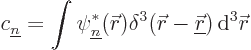
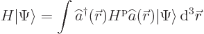
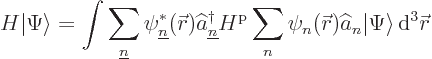
This example exercise from Srednicki [43, p. 11] uses quantum field theory to describe nonrelativistic quantum mechanics. It illustrates some of the mathematics that you will encounter in quantum field theories.
The objective is to convert the classical nonrelativistic Schrödinger
equation for ![]()
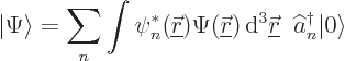
In quantum field theory, the wave function for exactly ![]()
The quantum amplitude of that ket state is the preceding ![]() ,
,
So far, all this gives just the ket for one particular set of particle positions. But then it is integrated over all possible particle positions.
The Fock space Schrödinger equation for ![]()
The goal is now to show that the Schrödinger equation (A.72) for
the Fock space ket ![]()
![]() .
.
Before trying to tackle this problem, it is probably a good idea to
review representations of functions using delta functions. As the
simplest example, a wave function ![]()
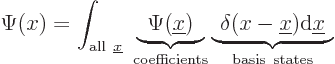
Now assume that ![]()
![]()
![]() ,
,
![\begin{eqnarray*}
H_1 \Psi(x)
& = &
\int_{{\rm all }{\underline x}}
H_1\Psi...
...})
\right]
\delta(x - {\underline x})
{ \rm d}{\underline x}
\end{eqnarray*}](img4105.gif)
You may be surprised by this, because if you straightforwardly apply
the Hamiltonian ![]() ,
,![]() ,
,![]() ,
,
![\begin{displaymath}
H_1 \Psi(x) =
\int_{{\rm all }{\underline x}}
\Psi({\und...
...) \delta(x - {\underline x})
\right]
{ \rm d}{\underline x}
\end{displaymath}](img4106.gif)
However, the two expressions are indeed the same. Whether there is an
![]()
![]()
![]()
![]()
![]() .
.![]() .
.![]()
![]()
The bottom line is that you do not want to use the expression in which the Hamiltonian is applied to the basis states, because derivatives of delta functions are highly singular objects that you should not touch with a ten foot pole. (And if you have mathematical integrity, you would not really want to use delta functions either. At least not the way that they do it in physics. But in that case, you better forget about quantum field theory.)
It may here be noted that if you do have to differentiate an integral
for a function ![]()
![]()
![]()
![]() ,
,
Still, there is an important observation here: you might either know what an operator does to the coefficients, leaving the basis states untouched, or what it does to the basis states, leaving the coefficients untouched. Either one will tell you the final effect of the operator, but the mathematics is different.
Now that the general terms of engagement have been discussed, it is
time to start solving Srednicki’s problem. The Fock space wave
function ket can be thought of the same way as the example:

Note that Fock states do not know about particle numbers. A Fock
basis state is the same regardless what the classical wave function
calls the particles. It means that the same Fock basis state
ket reappears in the integration above at all swapped positions of the
particles. (For fermions read: the same except possibly a sign
change, since swapping the order of application of any two ![]()
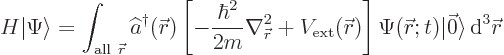
The left hand side of the Fock space Schrödinger equation (A.72) is
evaluated by pushing the time derivative inside the above integral for
![]() :
:

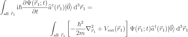
Applying the Fock-space Hamiltonian (A.73) on the wave
function is quite a different story, however. It is best to start
with just a single particle:


It is now that the (anti)commutator relations become useful. The fact
that for bosons ![]()
![]()
![]()
But when you swap the order of these operators, you get a factor
![]() .
.

Then, renotating ![]()
![]() ,
,
If there is more than one particle, however, the equivalent latter
conclusion is not justified. Remember that the same Fock space
kets reappear in the integration at swapped positions of the
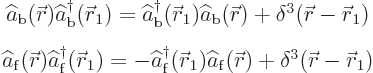
particles. It now makes a difference. The following example from
basic vectors illustrates the problem: yes, ![]()
![]()
![]()
![]()
![]()
![]() ,
,![]()
![]()
![]()
![]()
![]()
![]()
![]()
![]()
![]() ;
;![]()
![]()
![]() .
.![]()
![]()
![]()
![]()
![]()
![]() .
.
In any case, the problem has been solved for a system with one
particle. Doing it for ![]()

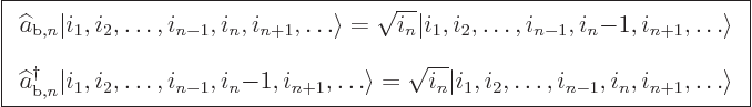
![\begin{displaymath}
\fbox{$\displaystyle
\left[\widehat a_{{\rm{b}},n},\wideha...
...rm{b}},{\underline n}}\right] = \delta_{n{\underline n}}
$} %
\end{displaymath}](img4041.gif)

![\begin{displaymath}
\fbox{$\displaystyle
\Big[\widehat a_{\rm{b}}({\skew0\vec ...
...g] = \delta^3({\skew0\vec r}-{\underline{\skew0\vec r}})
$} %
\end{displaymath}](img4074.gif)