A.2 An ex­am­ple of vari­a­tional cal­cu­lus

The prob­lem to solve in ad­den­dum {A.22.1} pro­vides a sim­ple ex­am­ple of vari­a­tional cal­cu­lus.

The prob­lem can be sum­ma­rized as fol­lows. Given is the fol­low­ing ex­pres­sion for the net en­ergy of a sys­tem:

$\parbox{400pt}{\hspace{11pt}\hfill$\displaystyle E = \frac{\epsilon_1}{2}\int ... ...w0\vec r} - \int \sigma_{\rm{p}} \varphi{ \rm d}^3{\skew0\vec r} $\hfill(1)}$

Here the op­er­a­tor $\nabla$ is de­fined as

$$\nabla \equiv {\hat\imath}\frac{\partial}{\partial x} + {\... ...phi}{\partial y} + {\hat k}\frac{\partial\varphi}{\partial z}$$

The in­te­grals are over all space, or over some other given re­gion. Fur­ther $\epsilon_1$ is as­sumed to be a given pos­i­tive con­stant and $\sigma_{\rm {p}}$ $\vphantom0\raisebox{1.5pt}{$=$}$ $\sigma_{\rm {p}}({\skew0\vec r})$ is a given func­tion of the po­si­tion ${\skew0\vec r}$. The func­tion $\varphi$ $\vphantom0\raisebox{1.5pt}{$=$}$ $\varphi({\skew0\vec r})$ will be called the po­ten­tial and is not given. Ob­vi­ously the en­ergy de­pends on what this po­ten­tial is. Math­e­mati­cians would say that $E$ is a “func­tional,” a num­ber that de­pends on what a func­tion is.

The en­ergy $E$ will be min­i­mal for some spe­cific po­ten­tial $\varphi_{\rm {min}}$. The ob­jec­tive is now to find an equa­tion for this po­ten­tial $\varphi_{\rm {min}}$ us­ing vari­a­tional cal­cu­lus.

To do so, the ba­sic idea is the fol­low­ing: imag­ine that you start at $\varphi_{\rm {min}}$ and then make an in­fin­i­tes­i­mally small change ${\rm d}\varphi$ to it. In that case there should be no change ${\rm d}{E}$ in en­ergy. Af­ter all, if there was an neg­a­tive change in $E$, then $E$ would de­crease. That would con­tra­dict that $\varphi_{\rm {min}}$ pro­duces the low­est en­ergy of all. If there was an pos­i­tive in­fin­i­tes­i­mal change in $E$, then a change in po­ten­tial of op­po­site sign would give a neg­a­tive change in $E$. Again that pro­duces a con­tra­dic­tion to what is given.

The typ­i­cal physi­cist would now work out the de­tails as fol­lows. The slightly per­turbed po­ten­tial is writ­ten as

$$\varphi({\skew0\vec r}) = \varphi_{\rm {min}}({\skew0\vec r}) + \delta\varphi({\skew0\vec r})$$

Note that the ${\rm d}$ in ${\rm d}\varphi$ has been reno­tated as $\delta$. That is be­cause every­one does so in vari­a­tional cal­cu­lus. The sym­bol does not make a dif­fer­ence, the idea re­mains the same. Note also that $\delta\varphi$ is a func­tion of po­si­tion; the change away from $\varphi_{\rm {min}}$ is nor­mally dif­fer­ent at dif­fer­ent lo­ca­tions. You are in fact al­lowed to choose any­thing you like for the func­tion $\delta\varphi$, as long as it is suf­fi­ciently small and it is zero at the lim­its of in­te­gra­tion.

Now just take dif­fer­en­tials like you typ­i­cally do it in cal­cu­lus or physics. If in cal­cu­lus you had some ex­pres­sion like $f^2$, you would say ${\rm d}{f^2}$ $\vphantom0\raisebox{1.5pt}{$=$}$ $2f{\rm d}{f}$. (For ex­am­ple, if $f$ is a func­tion of a vari­able $t$, then ${\rm d}{f^2}$$\raisebox{.5pt}{$/$}$​${\rm d}{t}$ $\vphantom0\raisebox{1.5pt}{$=$}$ $2f{\rm d}{f}$$\raisebox{.5pt}{$/$}$​${\rm d}{t}$. But physi­cists usu­ally do not bother with the ${\rm d}{t}$; then they do not have to worry what ex­actly $f$ is a func­tion of.) Sim­i­larly

$$\delta (\nabla\varphi)^2 = 2 (\nabla\varphi)\cdot \delta (\nabla\varphi)$$

where

$$\delta \nabla\varphi = \nabla(\varphi_{\rm {min}} + \delta\varphi) - \nabla(\varphi_{\rm {min}}) = \nabla\delta\varphi$$

so

$$\delta (\nabla\varphi)^2 = 2 (\nabla\varphi)\cdot(\nabla\delta\varphi)$$

For a change start­ing from $\varphi_{\rm {min}}$:

$$\delta (\nabla\varphi)^2 = 2 (\nabla\varphi_{\rm {min}})\cdot (\nabla\delta\varphi)$$

(Note that $\varphi$ by it­self gets ap­prox­i­mated as $\varphi_{\rm {min}}$, but $\delta\varphi$ is the com­pletely ar­bi­trary change that can be any­thing.) Also,

$$\delta(\sigma_{\rm {p}}\varphi) = \sigma_{\rm {p}}\delta\varphi$$

be­cause $\sigma_{\rm {p}}$ is a given con­stant at every po­si­tion.

To­tal you get for the change in en­ergy that must be zero

$\parbox{400pt}{\hspace{11pt}\hfill$\displaystyle 0 = \delta E = \frac{\epsilon... ... r} - \int \sigma_{\rm{p}} \delta\varphi{ \rm d}^3{\skew0\vec r} $\hfill(2)}$

A con­sci­en­tious math­e­mati­cian would shud­der at the above ma­nip­u­la­tions. And for good rea­son. Small changes are not good math­e­mat­i­cal con­cepts. There is no such thing as small in math­e­mat­ics. There are just lim­its where things go to zero. What a math­e­mati­cian would do in­stead is write the change in po­ten­tial as a some mul­ti­ple $\lambda$ of a cho­sen func­tion $\varphi_{\rm {c}}$. So the changed po­ten­tial is writ­ten as

$$\varphi({\skew0\vec r}) = \varphi_{\rm {min}}({\skew0\vec r}) + \lambda \varphi_{\rm {c}}({\skew0\vec r})$$

The cho­sen func­tion $\varphi_{\rm {c}}$ can still be any­thing that you want that van­ishes at the lim­its of in­te­gra­tion. But it is not as­sumed to be small. So now no math­e­mat­i­cal non­sense is writ­ten. The en­ergy for this changed po­ten­tial is

$$E = \frac{\epsilon_1}{2} \int [\nabla(\varphi_{\rm {min}} ... ...m {min}} + \lambda\varphi_{\rm {c}}) { \rm d}^3{\skew0\vec r}$$

Now this en­ergy is a func­tion of the mul­ti­ple $\lambda$. And that is a sim­ple nu­mer­i­cal vari­able. The en­ergy must be small­est at $\lambda$ = 0, be­cause $\varphi_{\rm {min}}$ gives the min­i­mum en­ergy. So the above func­tion of $\lambda$ must have a min­i­mum at $\lambda$ $\vphantom0\raisebox{1.5pt}{$=$}$ 0. That means that it must have a zero de­riv­a­tive at $\lambda$ $\vphantom0\raisebox{1.5pt}{$=$}$ 0. So just dif­fer­en­ti­ate the ex­pres­sion with re­spect to $\lambda$. (You can dif­fer­en­ti­ate as is, or sim­plify first and bring $\lambda$ out­side the in­te­grals.) Set this de­riv­a­tive to zero at $\lambda$ $\vphantom0\raisebox{1.5pt}{$=$}$ 0. That gives the same re­sult (2) as de­rived by physi­cists, ex­cept that $\varphi_{\rm {c}}$ takes the place of $\delta\varphi$. The re­sult is the same, but the de­riva­tion is nowhere fishy.

This de­riva­tion will re­turn to the no­ta­tions of physi­cists. The next step is to get rid of the de­riv­a­tives on $\delta\varphi$. Note that

$$\int (\nabla\varphi_{\rm {min}})\cdot(\nabla\delta\varphi) ... ...artial\delta\varphi}{\partial z} { \rm d}x {\rm d}y {\rm d}z$$

The way to get rid of the de­riv­a­tives on $\delta\varphi$ is by in­te­gra­tion by parts. In­te­gra­tion by parts pushes a de­riv­a­tive from one fac­tor on an­other. Here you see the real rea­son why the changes in po­ten­tial must van­ish at the lim­its of in­te­gra­tion. If they did not, in­te­gra­tions by parts would bring in con­tri­bu­tions from the lim­its of in­te­gra­tion. That would be a mess.

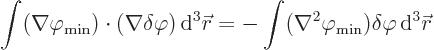
In­te­gra­tions by parts of the three terms in the in­te­gral in the $x$, $y$, and $z$ di­rec­tions re­spec­tively pro­duce

$$\int (\nabla\varphi_{\rm {min}})\cdot(\nabla\delta\varphi) ... ...n}}}{\partial z^2} \delta\varphi { \rm d}x {\rm d}y {\rm d}z$$

In vec­tor no­ta­tion, that be­comes

$$\int (\nabla\varphi_{\rm {min}})\cdot(\nabla\delta\varphi) ... ...la^2\varphi_{\rm {min}})\delta\varphi{ \rm d}^3{\skew0\vec r}$$

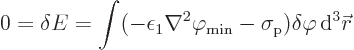
Sub­sti­tut­ing that in the change of en­ergy (2) gives

$$0 = \delta E = \int (-\epsilon_1\nabla^2\varphi_{\rm {min}}-\sigma_{\rm {p}}) \delta\varphi{ \rm d}^3{\skew0\vec r}$$

The fi­nal step is to say that this can only be true for what­ever change $\delta\varphi$ you take if the par­en­thet­i­cal ex­pres­sion is zero. That gives the fi­nal looked-for equa­tion for $\varphi_{\rm {min}}$:

$\parbox{400pt}{\hspace{11pt}\hfill$\displaystyle -\epsilon_1\nabla^2\varphi_{\rm{min}}-\sigma_{\rm{p}} = 0 $\hfill(3)}$

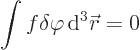
To jus­tify the above fi­nal step, call the par­en­thet­i­cal ex­pres­sion $f$ for short. Then the vari­a­tional state­ment above is of the form

$$\int f \delta\varphi { \rm d}^3{\skew0\vec r}= 0$$

where $\delta\varphi$ can be ar­bi­trar­ily cho­sen as long as it is zero at the lim­its of in­te­gra­tion. It is now to be shown that this im­plies that $f$ is every­where zero in­side the re­gion of in­te­gra­tion.

(Note here that what­ever func­tion $f$ is, it should not con­tain $\delta\varphi$. And there should not be any de­riv­a­tives of $\delta\varphi$ any­where at all. Oth­er­wise the above state­ment is not valid.)

The best way to see that $f$ must be zero every­where is first as­sume the op­po­site. As­sume that $f$ is nonzero at some point P. In that case se­lect a func­tion $\delta\varphi$ that is zero every­where ex­cept in a small vicin­ity of P, where it is pos­i­tive. (Make sure the vicin­ity is small enough that $f$ does not change sign in it.) Then the in­te­gral above is nonzero; in par­tic­u­lar, it will have the same sign as $f$ at P. But that is a con­tra­dic­tion, since the in­te­gral must be zero. So the func­tion $f$ can­not be nonzero at a point P; it must be zero every­where.

(There are more so­phis­ti­cated ways to do this. You could take $\delta\varphi$ as a pos­i­tive mul­ti­ple of $f$ that fades away to zero away from point P. In that case the in­te­gral will be pos­i­tive un­less $f$ is every­where zero. And sign changes in $f$ are no longer a prob­lem.)