| Quantum Mechanics for Engineers |
|
© Leon van Dommelen |
|
D.82 Classical spin-orbit derivation
This note derives the spin-orbit Hamiltonian from a more intuitive,
classical point of view than the Dirac equation mathematics.
Picture the magnetic electron as containing a pair of positive and
negative magnetic monopoles of a large strength  . The very
small distance from negative to positive pole is denoted by
. The very
small distance from negative to positive pole is denoted by  and the product

 is the magnetic dipole
strength, which is finite.
is the magnetic dipole
strength, which is finite.
Next imagine this electron smeared out in some orbit encircling the
nucleus with a speed  . The two poles will then be
smeared out into two parallel
. The two poles will then be
smeared out into two parallel magnetic currents
that
are very close together. The two currents have opposite directions
because the velocity of the poles is the same while their
charges are opposite. These magnetic currents will be encircled by
electric field lines just like the electric currents in figure
13.15 were encircled by magnetic field lines.
Now assume that seen from up very close, a segment of these currents
will seem almost straight and two-dimensional, so that two-dimensional analysis
can be used. Take a local coordinate system such that the
 -axis is aligned with the negative magnetic current and in
the direction of positive velocity. Rotate the
-axis is aligned with the negative magnetic current and in
the direction of positive velocity. Rotate the  -plane
around the -axis so that the positive current is to the right
of the negative one. The picture is then just like figure
13.15, except that the currents are magnetic and the field
lines electric. In this coordinate system, the vector from negative
to positive pole takes the form
-plane
around the -axis so that the positive current is to the right
of the negative one. The picture is then just like figure
13.15, except that the currents are magnetic and the field
lines electric. In this coordinate system, the vector from negative
to positive pole takes the form
 .
.
The magnetic current strength is defined as  , where
 is the moving magnetic charge per unit length of the current.
So, according to table 13.2 the negative current along
the -axis generates a two-dimensional electric field whose potential is
is the moving magnetic charge per unit length of the current.
So, according to table 13.2 the negative current along
the -axis generates a two-dimensional electric field whose potential is
To get the field of the positive current a distance  to the right
of it, shift
to the right
of it, shift  and change sign:
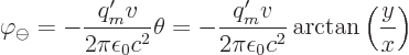
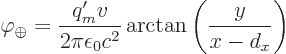
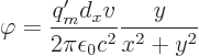
If these two potentials are added, the difference between the two
arctan functions can be approximated as  times the
derivative of the unshifted arctan. That can be seen from either
recalling the very definition of the partial derivative, or from
expanding the second arctan in a Taylor series in . The
bottom line is that the monopoles of the moving electron generate a
net electric field with a potential
times the
derivative of the unshifted arctan. That can be seen from either
recalling the very definition of the partial derivative, or from
expanding the second arctan in a Taylor series in . The
bottom line is that the monopoles of the moving electron generate a
net electric field with a potential
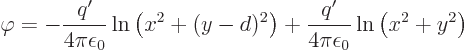
Now compare that with the electric field generated by a couple of
opposite electric line charges like in figure 13.12, a
negative one along the -axis and a positive one above it at a
position 
 . The electric dipole moment per
unit length of such a pair of line charges is by definition
. The electric dipole moment per
unit length of such a pair of line charges is by definition

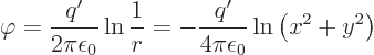
 , where
  is the
electric charge per unit length. According to table
13.1, a single electric charge along the -axis
creates an electric field whose potential is
is the
electric charge per unit length. According to table
13.1, a single electric charge along the -axis
creates an electric field whose potential is
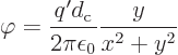
For an electric dipole consisting of a negative line charge along the
-axis and a positive one above it at ,
the field is then
and the difference between the two logarithms can be approximated as
 times the -derivative of the unshifted one. That
gives
times the -derivative of the unshifted one. That
gives
Comparing this with the potential of the monopoles, it is seen that
the magnetic currents create an electric dipole in the -direction
whose strength is 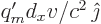 . And
since in this coordinate system the magnetic dipole moment is
. And
since in this coordinate system the magnetic dipole moment is

 and the velocity
 , it follows that the generated electric dipole strength
is
, it follows that the generated electric dipole strength
is
Since both dipole moments are per unit length, the same relation
applies between the actual magnetic dipole strength of the electron
and the electric dipole strength generated by its motion. The primes
can be omitted.
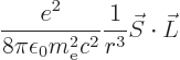
Now the energy of the electric dipole is  where
where
 is the electric field of the nucleus,


 according to table 13.1. So
the energy is:
according to table 13.1. So
the energy is:
and the order of the triple product of vectors can be changed and then
the angular momentum can be substituted:
To get the correct spin-orbit interaction, the magnetic dipole moment
used in this expression must be the classical one,


 . The additional factor
  2 for the
energy of the electron in a magnetic field does not apply here. There
does not seem to be a really good reason to give for that, except for
saying that the same Dirac equation that says that the additional
2 for the
energy of the electron in a magnetic field does not apply here. There
does not seem to be a really good reason to give for that, except for
saying that the same Dirac equation that says that the additional
 -factor is there in the magnetic interaction also says it is not in
the spin-orbit interaction. The expression for the energy becomes
-factor is there in the magnetic interaction also says it is not in
the spin-orbit interaction. The expression for the energy becomes
Getting rid of  using
using 
 , of
, of 
 using
using

 , and of
  using
using

 , the claimed expression
for the spin-orbit energy is found.
, the claimed expression
for the spin-orbit energy is found.