| Quantum Mechanics for Engineers |
|
© Leon van Dommelen |
|
D.57 The particle energy distributions
This note derives the Maxwell-Boltzmann, Fermi-Dirac, and
Bose-Einstein energy distributions of weakly interacting particles for
a system for which the net energy is precisely known.
The objective is to find the shelf numbers 

 for which the number of eigenfunctions
 is maximal. Actually, it is mathematically easier to
find the maximum of
is maximal. Actually, it is mathematically easier to
find the maximum of  , and that is the same
thing: if is as big as it can be, then so is
. The advantage of working with
is that it simplifies all the products in the
expressions for the derived in derivation
{D.56} into sums: mathematics says that
, and that is the same
thing: if is as big as it can be, then so is
. The advantage of working with
is that it simplifies all the products in the
expressions for the derived in derivation
{D.56} into sums: mathematics says that  equals
  plus
plus  for any (positive)
  and
and  .
.
It will be assumed, following derivation {N.24}, that if the
maximum value is found among all shelf occupation numbers,
whole numbers or not, it suffices. More daringly, errors less than a
particle are not going to be taken seriously.
In finding the maximum of , the shelf numbers
cannot be completely arbitrary; they are constrained by the conditions
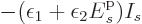
that the sum of the shelf numbers must equal the total number of
particles  , and that the particle energies must sum together
to the given total energy
, and that the particle energies must sum together
to the given total energy  :
:
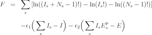
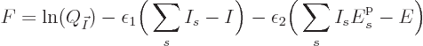
Mathematicians call this a constrained maximization problem.
According to calculus, without the constraints, you can just put the
derivatives of with respect to all the shelf
numbers  to zero to find the maximum. With the constraints, you
have to add
to zero to find the maximum. With the constraints, you
have to add penalty terms
that correct for any going
out of bounds, {D.48}, and the correct function whose
derivatives must be zero is
where the constants  and
and  are unknown penalty
factors called the Lagrangian multipliers.
are unknown penalty
factors called the Lagrangian multipliers.
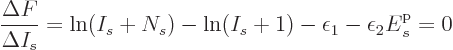
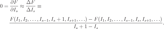
At the shelf numbers for which the number of eigenfunctions is
largest, the derivatives 

 must be zero.
However, that condition is difficult to apply exactly, because the
expressions for as given in the text involve the
factorial function, or rather, the gamma function. The gamma function
does not have a simple derivative. Here typical textbooks will flip
out the Stirling approximation of the factorial, but this
approximation is simply incorrect in parts of the range of interest,
and where it applies, the error is unknown.
must be zero.
However, that condition is difficult to apply exactly, because the
expressions for as given in the text involve the
factorial function, or rather, the gamma function. The gamma function
does not have a simple derivative. Here typical textbooks will flip
out the Stirling approximation of the factorial, but this
approximation is simply incorrect in parts of the range of interest,
and where it applies, the error is unknown.
It is a much better idea to approximate the differential quotient by a
difference quotient, as in
This approximation is very minor, since according to the so-called
mean value theorem of mathematics, the location where

 is zero is at most one particle away from
the desired location where is zero.
Better still,
is zero is at most one particle away from
the desired location where is zero.
Better still, 

 will be no more
that half a particle off, and the analysis already had to commit
itself to ignoring fractional parts of particles anyway. The
difference quotient leads to simple formulae because the gamma
function satisfies the condition
will be no more
that half a particle off, and the analysis already had to commit
itself to ignoring fractional parts of particles anyway. The
difference quotient leads to simple formulae because the gamma
function satisfies the condition 
 for any
value of
for any
value of  , compare the notations section under
!
.
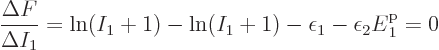
Now consider first distinguishable particles. The function  to
differentiate is defined above, and plugging in the expression for
to
differentiate is defined above, and plugging in the expression for
 as found in derivation {D.56} produces
For any value of the shelf number  , in the limit
 , tends to negative infinity because
  tends to positive infinity in that limit and its logarithm appears
with a minus sign. In the limit
tends to positive infinity in that limit and its logarithm appears
with a minus sign. In the limit  , tends
once more to negative infinity, since
, tends
once more to negative infinity, since  for large values of
is according to the so-called Stirling formula approximately
equal to
for large values of
is according to the so-called Stirling formula approximately
equal to 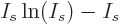 , so the
  term in goes
to minus infinity more strongly than the terms proportional to
might go to plus infinity. If tends to minus infinity at both
ends of the range
term in goes
to minus infinity more strongly than the terms proportional to
might go to plus infinity. If tends to minus infinity at both
ends of the range  1
1 
 , there must be
a maximum value of somewhere within that range where the
derivative with respect to is zero. More specifically, working
out the difference quotient:
, there must be
a maximum value of somewhere within that range where the
derivative with respect to is zero. More specifically, working
out the difference quotient:
and 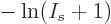 is infinity at 1 and minus infinity at
. Somewhere in between,
will cross zero. In particular, combining
the logarithms and then taking an exponential, the best estimate for
the shelf occupation number is
is infinity at 1 and minus infinity at
. Somewhere in between,
will cross zero. In particular, combining
the logarithms and then taking an exponential, the best estimate for
the shelf occupation number is
The correctness of the final half particle is clearly doubtful within
the made approximations. In fact, it is best ignored since it only
makes a difference at high energies where the number of particles per
shelf becomes small, and surely, the correct probability of finding a
particle must go to zero at infinite energies, not to minus half a
particle! Therefore, the best estimate 
 for the number of particles per
single-particle energy state becomes the Maxwell-Boltzmann
distribution. Note that the derivation might be off by a particle for
the lower energy shelves. But there are a lot of particles in a
macroscopic system, so it is no big deal.
for the number of particles per
single-particle energy state becomes the Maxwell-Boltzmann
distribution. Note that the derivation might be off by a particle for
the lower energy shelves. But there are a lot of particles in a
macroscopic system, so it is no big deal.
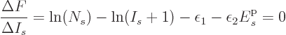
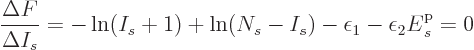
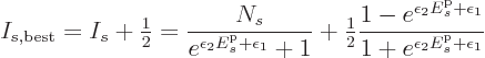
The case of identical fermions is next. The function to differentiate
is now
This time is minus infinity when a shelf number reaches
1 or  . So there must be a maximum to
when varies between those limits. The difference quotient
approximation produces
. So there must be a maximum to
when varies between those limits. The difference quotient
approximation produces
which can be solved to give
The final term, less than half a particle, is again best left away, to
ensure that 0  as it should. That gives
the Fermi-Dirac distribution.
as it should. That gives
the Fermi-Dirac distribution.
Finally, the case of identical bosons, is, once more, the tricky one.
The function to differentiate is now
For now, assume that  1 for all shelves. Then is again
minus infinity for 1. For
1 for all shelves. Then is again
minus infinity for 1. For  ,
however, will behave like
,
however, will behave like
 . This tends to minus
infinity if
. This tends to minus
infinity if  is positive, so for now
assume it is. Then the difference quotient approximation produces
is positive, so for now
assume it is. Then the difference quotient approximation produces
which can be solved to give
The final half particle is again best ignored to get the number of
particles to become zero at large energies. Then, if it is assumed
that the number of single-particle states on the shelves is
large, the Bose-Einstein distribution is obtained. If is not
large, the number of particles could be less than the predicted one by
up to a factor 2, and if is one, the entire story comes part.
And so it does if is not positive.
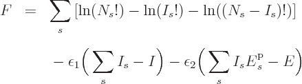
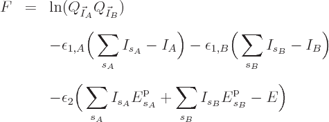
Before addressing these nasty problems, first the physical meaning of
the Lagrangian multiplier needs to be established. It
can be inferred from examining the case that two different systems,
call them  and
and  , are in thermal contact. Since the
interactions are assumed weak, the eigenfunctions of the combined
system are the products of those of the separate systems. That means
that the number of eigenfunctions of the combined system
, are in thermal contact. Since the
interactions are assumed weak, the eigenfunctions of the combined
system are the products of those of the separate systems. That means
that the number of eigenfunctions of the combined system
 is the product of those of the individual
systems. Therefore the function to differentiate becomes
is the product of those of the individual
systems. Therefore the function to differentiate becomes
Note the constraints: the number of particles in system must be
the correct number  of particles in that system, and similar for
system . However, since the systems are in thermal contact,
they can exchange energy through the weak interactions and there is no
longer a constraint on the energy of the individual systems. Only the
combined energy must equal the given total. That means the two
systems share the same Lagrangian variable . For
the rest, the equations for the two systems are just like if they were
not in thermal contact, because the logarithm in separates, and
then the differentiations with respect to the shelf numbers
of particles in that system, and similar for
system . However, since the systems are in thermal contact,
they can exchange energy through the weak interactions and there is no
longer a constraint on the energy of the individual systems. Only the
combined energy must equal the given total. That means the two
systems share the same Lagrangian variable . For
the rest, the equations for the two systems are just like if they were
not in thermal contact, because the logarithm in separates, and
then the differentiations with respect to the shelf numbers  and
and  give the same results as before.
It follows that two systems that have the same value of
can be brought into thermal contact and nothing happens,
macroscopically. However, if two systems with different values of
are brought into contact, the systems will adjust, and
energy will transfer between them, until the two values
have become equal. That means that is a temperature
variable. From here on, the temperature will be defined as  = 1/
= 1/ , so that
1/
, so that
1/ , with
  the Boltzmann constant. The same way,
for now the chemical potential
the Boltzmann constant. The same way,
for now the chemical potential  will simply be defined to be the
constant
will simply be defined to be the
constant  . Chapter 11.14.4
will eventually establish that the temperature defined here is the
ideal gas temperature, while derivation {D.61} will
establish that is the Gibbs free energy per atom that is
normally defined as the chemical potential.
. Chapter 11.14.4
will eventually establish that the temperature defined here is the
ideal gas temperature, while derivation {D.61} will
establish that is the Gibbs free energy per atom that is
normally defined as the chemical potential.
Returning now to the nasty problems of the distribution for bosons,
first assume that every shelf has at least two states, and that
 is positive even for the ground state. In that
case there is no problem with the derived solution. However,
Bose-Einstein condensation will occur when either the number density
is increased by putting more particles in the system, or the
temperature is decreased. Increasing particle density is associated
with increasing chemical potential because
is positive even for the ground state. In that
case there is no problem with the derived solution. However,
Bose-Einstein condensation will occur when either the number density
is increased by putting more particles in the system, or the
temperature is decreased. Increasing particle density is associated
with increasing chemical potential because
implies that every shelf particle number increases when
increases. Decreasing temperature by itself decreases the number of
particles, and to compensate and keep the number of particles the
same, must then once again increase. When gets very close
to the ground state energy, the exponential in the expression for the
number of particles on the ground state shelf 1 becomes very
close to one, making the total denominator very close to zero, so the
number of particles  in the ground state blows up. When it
becomes a finite fraction of the total number of particles even
when is macroscopically large, Bose-Einstein condensation is said
to have occurred.
in the ground state blows up. When it
becomes a finite fraction of the total number of particles even
when is macroscopically large, Bose-Einstein condensation is said
to have occurred.
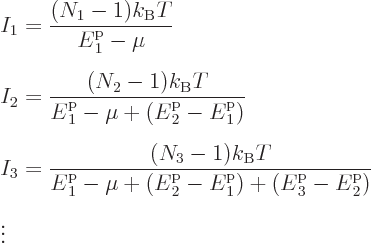
Note that under reasonable assumptions, it will only be the ground
state shelf that ever acquires a finite fraction of the particles.
For, assume the contrary, that shelf 2 also holds a finite
fraction of the particles. Using Taylor series expansion of the
exponential for small values of its argument, the shelf occupation
numbers are
For  to also be a finite fraction of the total number of
particles,
to also be a finite fraction of the total number of
particles,  must be similarly small as
  .
But then, reasonably assuming that the energy levels are at least
roughly equally spaced, and that the number of states will not
decrease with energy, so must
.
But then, reasonably assuming that the energy levels are at least
roughly equally spaced, and that the number of states will not
decrease with energy, so must  be a finite fraction of the total,
and so on. You cannot have a large number of shelves each having a
finite fraction of the particles, because there are not so many
particles. More precisely, a sum roughly like
be a finite fraction of the total,
and so on. You cannot have a large number of shelves each having a
finite fraction of the particles, because there are not so many
particles. More precisely, a sum roughly like
 , (or worse), sums to
an amount that is much larger than the term for 2 alone. So
if would be a finite fraction of , then the sum would
be much larger than .
, (or worse), sums to
an amount that is much larger than the term for 2 alone. So
if would be a finite fraction of , then the sum would
be much larger than .
What happens during condensation is that becomes much closer to
 than is to the next energy level
  , and
only the ground state shelf ends up with a finite fraction of the
particles. The remainder is spread out so much that the shelf numbers
immediately above the ground state only contain a negligible fraction
of the particles. It also follows that for all shelves except the
ground state one, may be approximated as being .
(Specific data for particles in a box is given in chapter
11.14.1. The entire story may of course need to be modified
in the presence of confinement, compare chapter 6.12.)
, and
only the ground state shelf ends up with a finite fraction of the
particles. The remainder is spread out so much that the shelf numbers
immediately above the ground state only contain a negligible fraction
of the particles. It also follows that for all shelves except the
ground state one, may be approximated as being .
(Specific data for particles in a box is given in chapter
11.14.1. The entire story may of course need to be modified
in the presence of confinement, compare chapter 6.12.)
The other problem with the analysis of the occupation numbers for
bosons is that the number of single-particle states on the shelves had
to be at least two. There is no reason why a system of
weakly-interacting spinless bosons could not have a unique
single-particle ground state. And combining the ground state with the
next one on a single shelf is surely not an acceptable approximation
in the presence of potential Bose-Einstein condensation. Fortunately,
the mathematics still partly works:
implies that  0. In other words,
is equal to the ground state energy exactly, rather than just
extremely closely as above.
0. In other words,
is equal to the ground state energy exactly, rather than just
extremely closely as above.
That then is the condensed state. Without a chemical potential that
can be adjusted, for any given temperature the states above the ground
state contain a number of particles that is completely unrelated to
the actual number of particles that is present. Whatever is left can
be dumped into the ground state, since there is no constraint on
.
Condensation stops when the number of particles in the states above
the ground state wants to become larger than the actual number of
particles present. Now the mathematics changes, because nature says
“Wait a minute, there is no such thing as a negative number of
particles in the ground state!” Nature now adds the constraint
that 0 rather than negative. That adds another penalty term,
 to and
  takes care of satisfying the
equation for the ground state shelf number. It is a sad story,
really: below the condensation temperature, the ground state was awash
in particles, above it, it has zero. None.
takes care of satisfying the
equation for the ground state shelf number. It is a sad story,
really: below the condensation temperature, the ground state was awash
in particles, above it, it has zero. None.
A system of weakly interacting helium atoms, spinless bosons, would
have a unique single-particle ground state like this. Since below the
condensation temperature, the elevated energy states have no clue
about an impending lack of particles actually present, physical
properties such as the specific heat stay analytical until
condensation ends.
It may be noted that above the condensation temperature it is only the
most probable set of the occupation numbers that have exactly zero
particles in the unique ground state. The expectation value of the
number in the ground state will include neighboring sets of occupation
numbers to the most probable one, and the number has nowhere to go but
up, compare {D.61}.
![\begin{displaymath}
F = \ln(I!) + \sum_s\left[I_s\ln(N_s)-\ln(I_s!)\right]
- \...
...epsilon_2 \bigg(\sum_s I_s {\vphantom' E}^{\rm p}_s - E\bigg)
\end{displaymath}](img7166.gif)