| Quantum Mechanics for Engineers |
|
© Leon van Dommelen |
|
Subsections
D.3 Lagrangian mechanics
This note gives the derivations for the addendum on the Lagrangian
equations of motion.
D.3.1 Lagrangian equations of motion
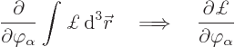
To derive the nonrelativistic Lagrangian, consider the system to be
build up from elementary particles numbered by an index  .
You may think of these particles as the atoms you would use if you
would do a molecular dynamics computation of the system. Because the
system is assumed to be fully determined by the generalized
coordinates, the position of each individual particle is fully fixed
by the generalized coordinates and maybe time. (For example, it is
implicit in a solid body approximation that the atoms are held rigidly
in their relative position. Of course, that is approximate; you pay
some price for avoiding a full molecular dynamics simulation.)
.
You may think of these particles as the atoms you would use if you
would do a molecular dynamics computation of the system. Because the
system is assumed to be fully determined by the generalized
coordinates, the position of each individual particle is fully fixed
by the generalized coordinates and maybe time. (For example, it is
implicit in a solid body approximation that the atoms are held rigidly
in their relative position. Of course, that is approximate; you pay
some price for avoiding a full molecular dynamics simulation.)
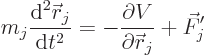
Newton’s second law says that the motion of each individual
particle is governed by
where the derivative of the potential  can be taken to be its
gradient, if you (justly) object to differentiating with respect to
vectors, and
can be taken to be its
gradient, if you (justly) object to differentiating with respect to
vectors, and  indicates any part of the force not described
by the potential.
indicates any part of the force not described
by the potential.
Now consider an infinitesimal virtual displacement of the system from
its normal evolution in time. It produces an infinitesimal change in
position  for each particle. After such a
displacement,
for each particle. After such a
displacement,  of course no longer satisfies
the correct equations of motion, but the kinetic and potential
energies still exist.
of course no longer satisfies
the correct equations of motion, but the kinetic and potential
energies still exist.
In the equation of motion for the correct position  above, take
the mass times acceleration to the other side, multiply by the virtual
displacement, sum over all particles , and integrate over an
arbitrary time interval:
above, take
the mass times acceleration to the other side, multiply by the virtual
displacement, sum over all particles , and integrate over an
arbitrary time interval:
Multiply out and integrate the first term by parts:
The virtual displacements of interest here are only nonzero over a
limited range of times, so the integration by parts did not produce
any end point values.
Recognize the first two terms within the brackets as the virtual
change in the Lagrangian due to the virtual displacement at that time.
Note that this requires that the potential energy depends only on the
position coordinates and time, and not also on the time derivatives of
the position coordinates. You get
![\begin{displaymath}
0 = \delta \int_{t_1}^{t_2} {\cal L}{ \rm d}t
+ \int_{t_1...
...j \left[\vec F'_j\cdot\delta{\skew0\vec r}_j\right] { \rm d}t
\end{displaymath}](img5852.gif) |
(D.3) |
In case that the additional forces are zero, this produces
the action principle: the time integral of the Lagrangian is unchanged
under infinitesimal virtual displacements of the system, assuming that
they vanish at the end points of integration. More generally, for the
virtual work by the additional forces to be zero will require that the
virtual displacements respect the rigid constraints, if any. The
infinite work done in violating a rigid constraint is not modeled by
the potential in any normal implementation.
Unchanging action is an integral equation involving the Lagrangian.
To get ordinary differential equations, take the virtual change in
position to be that due to an infinitesimal change  in
a single generic generalized coordinate. Represent the change in the
Lagrangian in the expression above by its partial derivatives, and the
same for
in
a single generic generalized coordinate. Represent the change in the
Lagrangian in the expression above by its partial derivatives, and the
same for  :
:
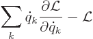
The integrand in the final term is by definition the generalized force
 multiplied by
  . In the first integral, the
second term can be integrated by parts, and then the integrals can be
combined to give
. In the first integral, the
second term can be integrated by parts, and then the integrals can be
combined to give
Now suppose that there is any time at which the expression within the
square brackets is nonzero. Then a virtual change that
is only nonzero in a very small time interval around that time, and
everywhere positive in that small interval, would produce a nonzero
right hand side in the above equation, but it must be zero. Therefore,
the expression within brackets must be zero at all times. That gives
the Lagrangian equations of motion, because the expression between
parentheses is defined as the canonical momentum.
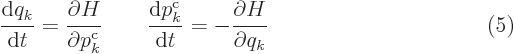
D.3.2 Hamiltonian dynamics
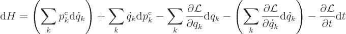
To derive the Hamiltonian equations, consider the general differential
of the Hamiltonian function (regardless of any motion that may go on).
According to the given definition of the Hamiltonian function, and
using a total differential for  ,
,
The sums within parentheses cancel each other because of the
definition of the canonical momentum. The remaining differences are
of the arguments of the Hamiltonian function, and so by the very
definition of partial derivatives,
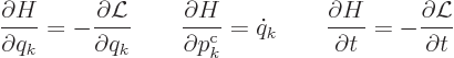
Now consider an actual motion. For an actual motion,  is
the time derivative of
is
the time derivative of  , so the second partial derivative
gives the first Hamiltonian equation of motion. The first partial
derivative gives the second equation when combined with the Lagrangian
equation of motion (A.2).
, so the second partial derivative
gives the first Hamiltonian equation of motion. The first partial
derivative gives the second equation when combined with the Lagrangian
equation of motion (A.2).
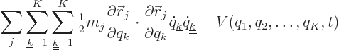
It is still to be shown that the Hamiltonian of a classical system is
the sum of kinetic and potential energy if the position of the system
does not depend explicitly on time. The Lagrangian can be written out
in terms of the system particles as
where the sum represents the kinetic energy. The Hamiltonian is
defined as
and straight substitution shows the first term to be twice the kinetic
energy.
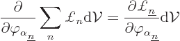
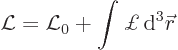
D.3.3 Fields
As discussed in {A.1.5}, the Lagrangian for fields
takes the form
Here the spatial integration is over all space. The first term
depends only on the discrete variables
where 
 denotes discrete variable number
  .
The dot indicates the time derivative of that variable. The
Lagrangian density also depends on the fields
.
The dot indicates the time derivative of that variable. The
Lagrangian density also depends on the fields
where  is field number
  . A subscript
 indicates the partial time derivative, and 1, 2, or 3 the partial
 ,
,  or
or  derivative.
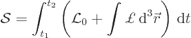
The action is
where the time range from  to
to  must include the times of
interest. The action must be unchanged under small deviations from
the correct evolution, as long as these deviations vanish at the
limits of integration. That requirement defines the Lagrangian. (For
simple systems the Lagrangian then turns out to be the difference
between kinetic and potential energies. But it is not obvious what to
make of that if there are fields.)
must include the times of
interest. The action must be unchanged under small deviations from
the correct evolution, as long as these deviations vanish at the
limits of integration. That requirement defines the Lagrangian. (For
simple systems the Lagrangian then turns out to be the difference
between kinetic and potential energies. But it is not obvious what to
make of that if there are fields.)
Consider now first an infinitesimal deviation
in a discrete variable . The change in
action that must be zero is then
After an integration by parts of the second and fourth terms that
becomes, noting that the deviation must vanish at the initial and
final times,
This can only be zero for whatever you take
if the expression within square brackets
is zero. That gives the final Lagrangian equation for the discrete
variable as
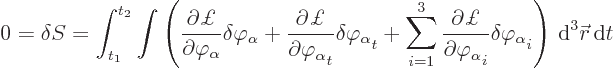
Next consider an infinitesimal deviation 
 in field . The
change in action that must be zero is then
in field . The
change in action that must be zero is then
Now integrate the derivative terms by parts in the appropriate
direction to get, noting that the deviation must vanish at the limits
of integration,
Here  for
for  1, 2, or 3 stands for , ,
or . If the above expression is to be zero for whatever you
take the small change
to be, then the expression within square
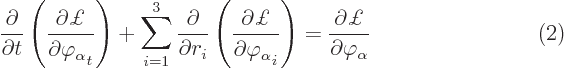
brackets will have to be zero at every position and time. That gives
the equation for the field :
1, 2, or 3 stands for , ,
or . If the above expression is to be zero for whatever you
take the small change
to be, then the expression within square
brackets will have to be zero at every position and time. That gives
the equation for the field :
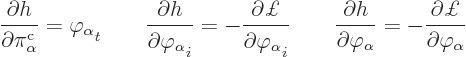
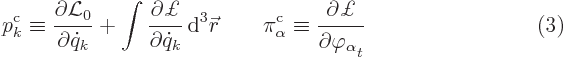
The canonical momenta are defined as
These are the quantities inside the time derivatives of the Lagrangian
equations.
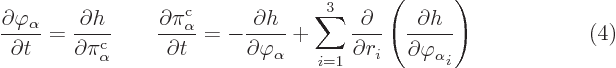
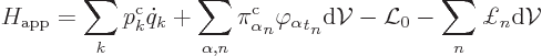
For Hamilton’s equations, assume at first that there are no
discrete variables. In that case, the Hamiltonian can be written in
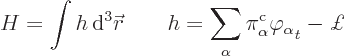
terms of a Hamiltonian density  :
:
Take a differential of the Hamiltonian density
The first and third terms in the square brackets cancel because of the
definition of the canonical momentum. Then according to calculus
The first of these expressions gives the time derivative of
. The other expressions may be used to replace
the derivatives of the Lagrangian density in the Lagrangian equations
of motion (2). That gives Hamilton’s equations as
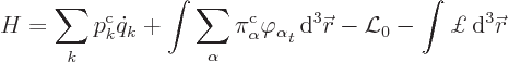
If there are discrete variables, this no longer works. The full
Hamiltonian is then
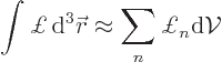
To find Hamilton’s equations, the integrals in this Hamiltonian
must be approximated. The region of integration is mentally chopped
into little pieces of the same volume  . Then by
approximation
. Then by
approximation
Here  numbers the small pieces and
  stands for the value of
 at the center point of piece . Note that this is
essentially the Riemann sum of calculus. A similar approximation is
made for the other integral in the Hamiltonian, and the one in the
canonical momenta (3). Then the approximate Hamiltonian becomes
at the center point of piece . Note that this is
essentially the Riemann sum of calculus. A similar approximation is
made for the other integral in the Hamiltonian, and the one in the
canonical momenta (3). Then the approximate Hamiltonian becomes
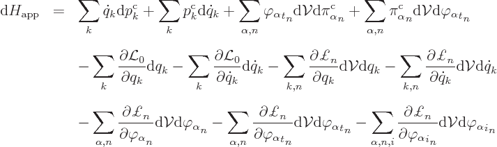
The differential of this approximate Hamiltonian is
The  and
and  terms drop
out because of the definitions of the canonical momenta. The
remainder allows expressions for the partial derivatives of the
approximate Hamiltonian to be identified.
terms drop
out because of the definitions of the canonical momenta. The
remainder allows expressions for the partial derivatives of the
approximate Hamiltonian to be identified.
The  term allows the time derivative of to be
identified with the partial derivative of
term allows the time derivative of to be
identified with the partial derivative of  with respect
to
with respect
to  . And the Lagrangian expression for the time
derivative of , as given in (1), may be rewritten
in terms of corresponding derivatives of the approximate Hamiltonian.
Together that gives, in the limit
. And the Lagrangian expression for the time
derivative of , as given in (1), may be rewritten
in terms of corresponding derivatives of the approximate Hamiltonian.
Together that gives, in the limit  ,
,
For the field, consider an position  corresponding to the center
of an arbitrary little volume
corresponding to the center
of an arbitrary little volume  . Then the
 term allows the time derivative of
at this arbitrary position to be identified in terms
of the partial derivative of the approximate Hamiltonian with respect
to
term allows the time derivative of
at this arbitrary position to be identified in terms
of the partial derivative of the approximate Hamiltonian with respect
to  at the same location. And the Lagrangian
expression for the time derivative of , as
given by (2), may be rewritten in terms of corresponding derivatives
of the approximate Hamiltonian. Together that gives, in the limit
, and leaving away since it can be any
position,
at the same location. And the Lagrangian
expression for the time derivative of , as
given by (2), may be rewritten in terms of corresponding derivatives
of the approximate Hamiltonian. Together that gives, in the limit
, and leaving away since it can be any
position,
Of course, in real life you would not actually write out these limits.
Instead you simply differentiate the normal Hamiltonian  until you
have to start differentiating inside an integral, like maybe,
until you
have to start differentiating inside an integral, like maybe,
Then you think to yourself that you are not really evaluating this,
but actually
where indicates the position that you are considering the field
at. And you are going to divide out the volume . That
then boils down to
even though the left hand side would mathematically be nonsense
without discretization and division by .
![\begin{displaymath}
0 = \int_{t_1}^{t_2} \sum_j \left[- m_j \frac{{\rm d}^2 {\s...
...r}_j}
+ \vec F'_j\right]\cdot\delta{\skew0\vec r}_j{ \rm d}t
\end{displaymath}](img5850.gif)
![\begin{displaymath}
0 = \int_{t_1}^{t_2} \sum_j
\left[
m_j \frac{{\rm d}{\ske...
... r}_j
+ \vec F'_j \delta {\skew0\vec r}_j
\right] { \rm d}t
\end{displaymath}](img5851.gif)
![\begin{displaymath}
0 =
\int_{t_1}^{t_2}
\left[
\frac{\partial{\cal L}}{\par...
...ial{\skew0\vec r}_j}{\partial q_k}\delta q_k\right] { \rm d}t
\end{displaymath}](img5855.gif)
![\begin{displaymath}
0 =
\int_{t_1}^{t_2}
\left[
\frac{\partial{\cal L}}{\par...
...{\partial\dot q_k}\right)
+ Q_k
\right]\delta q_k { \rm d}t
\end{displaymath}](img5856.gif)

![\begin{displaymath}
0 = \delta{\cal S}=
\int_{t_1}^{t_2} \left[
\frac{\partia...
...q}_k} { \rm d}^3{\skew0\vec r}
\right] \delta q_k { \rm d}t
\end{displaymath}](img5866.gif)

![\begin{displaymath}
0 = \delta S = \int_{t_1}^{t_2} \int \left[
\frac{\partial...
...ight] \delta\varphi_\alpha { \rm d}^3{\skew0\vec r}{ \rm d}t
\end{displaymath}](img5871.gif)
![\begin{displaymath}
{\rm d}h = \sum_\alpha \left[
\pi^{\rm {c}}_\alpha {\rm d}...
...ounds }{\partial\varphi_\alpha} {\rm d}\varphi_\alpha
\right]
\end{displaymath}](img5875.gif)