4.4 Ex­pec­ta­tion Value and Stan­dard De­vi­a­tion

It is a strik­ing con­se­quence of quan­tum me­chan­ics that phys­i­cal quan­ti­ties may not have a value. This oc­curs when­ever the wave func­tion is not an eigen­func­tion of the quan­tity of in­ter­est. For ex­am­ple, the ground state of the hy­dro­gen atom is not an eigen­func­tion of the po­si­tion op­er­a­tor ${\widehat x}$, so the $x$-​po­si­tion of the elec­tron does not have a value. Ac­cord­ing to the or­tho­dox in­ter­pre­ta­tion, it can­not be pre­dicted with cer­tainty what a mea­sure­ment of such a quan­tity will pro­duce.

How­ever, it is pos­si­ble to say some­thing if the same mea­sure­ment is done on a large num­ber of sys­tems that are all the same be­fore the mea­sure­ment. An ex­am­ple would be $x$-​po­si­tion mea­sure­ments on a large num­ber of hy­dro­gen atoms that are all in the ground state be­fore the mea­sure­ment. In that case, it is rel­a­tively straight­for­ward to pre­dict what the av­er­age, or ex­pec­ta­tion value, of all the mea­sure­ments will be.

The ex­pec­ta­tion value is cer­tainly not a re­place­ment for the clas­si­cal value of phys­i­cal quan­ti­ties. For ex­am­ple, for the hy­dro­gen atom in the ground state, the ex­pec­ta­tion po­si­tion of the elec­tron is in the nu­cleus by sym­me­try. Yet be­cause the nu­cleus is so small, mea­sure­ments will never find it there! (The typ­i­cal mea­sure­ment will find it a dis­tance com­pa­ra­ble to the Bohr ra­dius away.) Ac­tu­ally, that is good news, be­cause if the elec­tron would be in the nu­cleus as a clas­si­cal par­ti­cle, its po­ten­tial en­ergy would be al­most mi­nus in­fin­ity in­stead of the cor­rect value of about -27 eV. It would be a very dif­fer­ent uni­verse. Still, hav­ing an ex­pec­ta­tion value is of course bet­ter than hav­ing no in­for­ma­tion at all.

The av­er­age dis­crep­ancy be­tween the ex­pec­ta­tion value and the ac­tual mea­sure­ments is called the stan­dard de­vi­a­tion.. In the hy­dro­gen atom ex­am­ple, where typ­i­cally the elec­tron is found a dis­tance com­pa­ra­ble to the Bohr ra­dius away from the nu­cleus, the stan­dard de­vi­a­tion in the $x$-​po­si­tion turns out to be ex­actly one Bohr ra­dius. (The same of course for the stan­dard de­vi­a­tions in the $y$ and $z$ po­si­tions away from the nu­cleus.)

In gen­eral, the stan­dard de­vi­a­tion is the quan­ti­ta­tive mea­sure for how much un­cer­tainty there is in a phys­i­cal value. If the stan­dard de­vi­a­tion is very small com­pared to what you are in­ter­ested in, it is prob­a­bly OK to use the ex­pec­ta­tion value as a clas­si­cal value. It is per­fectly fine to say that the elec­tron of the hy­dro­gen atom that you are mea­sur­ing is in your lab but it is not OK to say that it has count­less elec­tron volts of neg­a­tive po­ten­tial en­ergy be­cause it is in the nu­cleus.

This sec­tion dis­cusses how to find ex­pec­ta­tion val­ues and stan­dard de­vi­a­tions af­ter a brief in­tro­duc­tion to the un­der­ly­ing ideas of sta­tis­tics.

Key Points

$\begin{picture}(15,5.5)(0,-3) \put(2,0){\makebox(0,0){\scriptsize\bf0}} \put(12... ...\thicklines \put(3,0){\line(1,0){12}}\put(11.5,-2){\line(1,0){3}} \end{picture}$

The ex­pec­ta­tion value is the av­er­age value ob­tained when do­ing mea­sure­ments on a large num­ber of ini­tially iden­ti­cal sys­tems. It is as close as quan­tum me­chan­ics can come to hav­ing clas­si­cal val­ues for un­cer­tain phys­i­cal quan­ti­ties.

$\begin{picture}(15,5.5)(0,-3) \put(2,0){\makebox(0,0){\scriptsize\bf0}} \put(12... ...\thicklines \put(3,0){\line(1,0){12}}\put(11.5,-2){\line(1,0){3}} \end{picture}$

The stan­dard de­vi­a­tion is how far the in­di­vid­ual mea­sure­ments on av­er­age de­vi­ate from the ex­pec­ta­tion value. It is the quan­ti­ta­tive mea­sure of un­cer­tainty in quan­tum me­chan­ics.

4.4.1 Sta­tis­tics of a die

Since it seems to us hu­mans as if, in Ein­stein's words, God is play­ing dice with the uni­verse, it may be a worth­while idea to ex­am­ine the sta­tis­tics of a die first.

For a fair die, each of the six num­bers will, on av­er­age, show up a frac­tion 1/6 of the num­ber of throws. In other words, each face has a prob­a­bil­ity of 1/6.

The av­er­age value of a large num­ber of throws is called the ex­pec­ta­tion value. For a fair die, the ex­pec­ta­tion value is 3.5. Af­ter all, num­ber 1 will show up in about 1/6 of the throws, as will num­bers 2 through 6, so the av­er­age is

$$\frac{\mbox{(number of throws)}\times (\frac16 1+\frac16\... ...6 4+\frac16 5+\frac16 6)} {\mbox{number of throws}} = 3.5$$

The gen­eral rule to get the ex­pec­ta­tion value is to sum the prob­a­bil­ity for each value times the value. In this ex­am­ple:

$${\textstyle\frac{1}{6}} 1 + {\textstyle\frac{1}{6}} 2 + {... ... {\textstyle\frac{1}{6}} 5 + {\textstyle\frac{1}{6}} 6 = 3.5$$

Note that the name ex­pec­ta­tion value is very poorly cho­sen. Even though the av­er­age value of a lot of throws will be 3.5, you would surely not ex­pect to throw 3.5. But it is prob­a­bly too late to change the name now.

The max­i­mum pos­si­ble de­vi­a­tion from the ex­pec­ta­tion value does of course oc­cur when you throw a 1 or a 6; the ab­solute de­vi­a­tion is then $\vert 1-3.5\vert$ $\vphantom0\raisebox{1.5pt}{$=$}$ $\vert 6-3.5\vert$ $\vphantom0\raisebox{1.5pt}{$=$}$ 2.5. It means that the pos­si­ble val­ues pro­duced by a throw can de­vi­ate as much as 2.5 from the ex­pec­ta­tion value.

How­ever, the max­i­mum pos­si­ble de­vi­a­tion from the av­er­age is not a use­ful con­cept for quan­ti­ties like po­si­tion, or for the en­ergy lev­els of the har­monic os­cil­la­tor, where the pos­si­ble val­ues ex­tend all the way to in­fin­ity. So, in­stead of the max­i­mum de­vi­a­tion from the ex­pec­ta­tion value, some av­er­age de­vi­a­tion is bet­ter. The most use­ful of those is called the “stan­dard de­vi­a­tion”, de­noted by $\sigma$. It is found in two steps: first the av­er­age square de­vi­a­tion from the ex­pec­ta­tion value is com­puted, and then a square root is taken of that. For the die that works out to be:

$$\begin{eqnarray*} \sigma & = & \big[ {\textstyle\frac{1}{6}}(1-3.5)^2+{\textst... ...^2+{\textstyle\frac{1}{6}}(6-3.5)^2 \big]^{1/2} \\ & = & 1.71 \end{eqnarray*}$$

On av­er­age then, the throws are 1.71 points off from 3.5.

Key Points

$\begin{picture}(15,5.5)(0,-3) \put(2,0){\makebox(0,0){\scriptsize\bf0}} \put(12... ...\thicklines \put(3,0){\line(1,0){12}}\put(11.5,-2){\line(1,0){3}} \end{picture}$

The ex­pec­ta­tion value is ob­tained by sum­ming the pos­si­ble val­ues times their prob­a­bil­i­ties.

$\begin{picture}(15,5.5)(0,-3) \put(2,0){\makebox(0,0){\scriptsize\bf0}} \put(12... ...\thicklines \put(3,0){\line(1,0){12}}\put(11.5,-2){\line(1,0){3}} \end{picture}$

To get the stan­dard de­vi­a­tion, first find the av­er­age square de­vi­a­tion from the ex­pec­ta­tion value, then take a square root of that.

4.4.1 Re­view Ques­tions

1.

Sup­pose you toss a coin a large num­ber of times, and count heads as one, tails as two. What will be the ex­pec­ta­tion value?

So­lu­tion esda-a

2.

Con­tin­u­ing this ex­am­ple, what will be the max­i­mum de­vi­a­tion?

So­lu­tion esda-b

3.

Con­tin­u­ing this ex­am­ple, what will be the stan­dard de­vi­a­tion?

So­lu­tion esda-c

4.

Have I got a die for you! By means of a small piece of lead in­te­grated into its light-weight struc­ture, it does away with that old-fash­ioned un­cer­tainty. It comes up six every time! What will be the ex­pec­ta­tion value of your throws? What will be the stan­dard de­vi­a­tion?

So­lu­tion esda-d

4.4.2 Sta­tis­tics of quan­tum op­er­a­tors

The ex­pec­ta­tion val­ues of the op­er­a­tors of quan­tum me­chan­ics are de­fined in the same way as those for the die.

Con­sider an ar­bi­trary phys­i­cal quan­tity, call it $a$, and as­sume it has an as­so­ci­ated op­er­a­tor $A$. For ex­am­ple, if the phys­i­cal quan­tity $a$ is the to­tal en­ergy $E$, $A$ will be the Hamil­ton­ian $H$.

The equiv­a­lent of the face val­ues of the die are the val­ues that the quan­tity $a$ can take, and ac­cord­ing to the or­tho­dox in­ter­pre­ta­tion, that are the eigen­val­ues

$$a_1, a_2, a_3, \ldots$$

of the op­er­a­tor $A$.

Next, the prob­a­bil­i­ties of get­ting those val­ues are ac­cord­ing to quan­tum me­chan­ics the square mag­ni­tudes of the co­ef­fi­cients when the wave func­tion is writ­ten in terms of the eigen­func­tions of $A$. In other words, if $\alpha_1$, $\alpha_2$, $\alpha_3$, ...are the eigen­func­tions of op­er­a­tor $A$, and the wave func­tion is

$$\Psi = c_1 \alpha_1 + c_2 \alpha_2 + c_3 \alpha_3 + \ldots$$

then $\vert c_1\vert^2$ is the prob­a­bil­ity of value $a_1$, $\vert c_2\vert^2$ the prob­a­bil­ity of value $a_2$, etcetera.

The ex­pec­ta­tion value is writ­ten as $\left\langle{a}\right\rangle$, or as $\left\langle{A}\right\rangle$, what­ever is more ap­peal­ing. Like for the die, it is found as the sum of the prob­a­bil­ity of each value times the value:

$$\left\langle{a}\right\rangle = \vert c_1\vert^2 a_1 + \vert c_2\vert^2 a_2 + \vert c_3\vert^2 a_3 + \ldots$$

Of course, the eigen­func­tions might be num­bered us­ing mul­ti­ple in­dices; that does not re­ally make a dif­fer­ence. For ex­am­ple, the eigen­func­tions $\psi_{nlm}$ of the hy­dro­gen atom are num­bered with three in­dices. In that case, if the wave func­tion of the hy­dro­gen atom is

$$\Psi = c_{100} \psi_{100}+ c_{200} \psi_{200}+ c_{210} \... ...psi_{211}+ c_{21-1} \psi_{21-1}+ c_{300} \psi_{300}+ \ldots$$

then the ex­pec­ta­tion value for en­ergy will be, not­ing that $E_1$ $\vphantom0\raisebox{1.5pt}{$=$}$ $\vphantom{0}\raisebox{1.5pt}{$-$}$13.6 eV, $E_2$ $\vphantom0\raisebox{1.5pt}{$=$}$ $\vphantom{0}\raisebox{1.5pt}{$-$}$3.4 eV, ...:

$$\left\langle{E}\right\rangle = - \vert c_{100}\vert^2 13.6... ....4 \mbox{ eV} - \vert c_{211}\vert^2 3.4 \mbox{ eV} - \ldots$$

Also, the ex­pec­ta­tion value of the square an­gu­lar mo­men­tum will be, re­call­ing that its eigen­val­ues are $l(l+1)\hbar^2$,

$$\langle L^2\rangle = \vert c_{100}\vert^2 0 + \vert c_{20... ... c_{21-1}\vert^2 2 \hbar^2 + \vert c_{300}\vert^2 0 + \ldots$$

Also, the ex­pec­ta­tion value of the $z$-​com­po­nent of an­gu­lar mo­men­tum will be, re­call­ing that its eigen­val­ues are $m\hbar$,

$$\langle L_z\rangle = \vert c_{100}\vert^2 0 + \vert c_{20... ...vert c_{21-1}\vert^2 \hbar + \vert c_{300}\vert^2 0 + \ldots$$

Key Points

$\begin{picture}(15,5.5)(0,-3) \put(2,0){\makebox(0,0){\scriptsize\bf0}} \put(12... ...\thicklines \put(3,0){\line(1,0){12}}\put(11.5,-2){\line(1,0){3}} \end{picture}$

The ex­pec­ta­tion value of a phys­i­cal quan­tity is found by sum­ming its eigen­val­ues times the prob­a­bil­ity of mea­sur­ing that eigen­value.

$\begin{picture}(15,5.5)(0,-3) \put(2,0){\makebox(0,0){\scriptsize\bf0}} \put(12... ...\thicklines \put(3,0){\line(1,0){12}}\put(11.5,-2){\line(1,0){3}} \end{picture}$

To find the prob­a­bil­i­ties of the eigen­val­ues, the wave func­tion $\Psi$ can be writ­ten in terms of the eigen­func­tions of the phys­i­cal quan­tity. The prob­a­bil­i­ties will be the square mag­ni­tudes of the co­ef­fi­cients of the eigen­func­tions.

4.4.2 Re­view Ques­tions

1.

The 2p$_x$ pointer state of the hy­dro­gen atom was de­fined as

$$\frac 1{\sqrt 2}\left(-\psi_{211}+\psi_{21-1}\right).$$

What are the ex­pec­ta­tion val­ues of en­ergy, square an­gu­lar mo­men­tum, and $z$ an­gu­lar mo­men­tum for this state?

So­lu­tion esdb-a

2.

Con­tin­u­ing the pre­vi­ous ques­tion, what are the stan­dard de­vi­a­tions in en­ergy, square an­gu­lar mo­men­tum, and $z$ an­gu­lar mo­men­tum?

So­lu­tion esdb-b

4.4.3 Sim­pli­fied ex­pres­sions

The pro­ce­dure de­scribed in the pre­vi­ous sec­tion to find the ex­pec­ta­tion value of a quan­tity is un­wieldy: it re­quires that first the eigen­func­tions of the quan­tity are found, and next that the wave func­tion is writ­ten in terms of those eigen­func­tions. There is a quicker way.

As­sume that you want to find the ex­pec­ta­tion value, $\left\langle{a}\right\rangle$ or $\left\langle{A}\right\rangle$, of some quan­tity $a$ with as­so­ci­ated op­er­a­tor $A$. The sim­pler way to do it is as an in­ner prod­uct:

$$\fbox{$\displaystyle \left\langle{A}\right\rangle = \langle \Psi\vert A \vert \Psi\rangle. $}$$ (4.43)

(Re­call that $\langle\Psi\vert A\vert\Psi\rangle$ is just the in­ner prod­uct $\langle\Psi\vert A\Psi\rangle$; the ad­di­tional sep­a­rat­ing bar is of­ten vi­su­ally con­ve­nient, though.) This for­mula for the ex­pec­ta­tion value is eas­ily re­mem­bered as leav­ing out $\Psi$ from the in­ner prod­uct bracket. The rea­son that $\langle\Psi\vert A\vert\Psi\rangle$ works for get­ting the ex­pec­ta­tion value is given in de­riva­tion {D.17}.

The sim­pli­fied ex­pres­sion for the ex­pec­ta­tion value can also be used to find the stan­dard de­vi­a­tion, $\sigma_A$ or $\sigma_a$:

$$\fbox{$\displaystyle \sigma_A = \sqrt{\langle(A - \left\langle{A}\right\rangle )^2\rangle} $} %$$ (4.44)

where $\left\langle{(A-\langle{A}\rangle)^2}\right\rangle$ is the in­ner prod­uct $\left\langle\vphantom{(A-\langle{A}\rangle)^2\Psi}\Psi\hspace{-\nulldelimitersp... ...3em}\right.\!\left\vert\vphantom{\Psi}(A-\langle{A}\rangle)^2\Psi\right\rangle$.

Key Points

$\begin{picture}(15,5.5)(0,-3) \put(2,0){\makebox(0,0){\scriptsize\bf0}} \put(12... ...\thicklines \put(3,0){\line(1,0){12}}\put(11.5,-2){\line(1,0){3}} \end{picture}$

The ex­pec­ta­tion value of a quan­tity $a$ with op­er­a­tor $A$ can be found as $\left\langle{A}\right\rangle$ $\vphantom0\raisebox{1.5pt}{$=$}$ $\left\langle\vphantom{A\Psi}\Psi\hspace{-\nulldelimiterspace}\hspace{.03em}\right.\!\left\vert\vphantom{\Psi}A\Psi\right\rangle$.

$\begin{picture}(15,5.5)(0,-3) \put(2,0){\makebox(0,0){\scriptsize\bf0}} \put(12... ...\thicklines \put(3,0){\line(1,0){12}}\put(11.5,-2){\line(1,0){3}} \end{picture}$

Sim­i­larly, the stan­dard de­vi­a­tion can be found us­ing the ex­pres­sion $\sigma_A$ $\vphantom0\raisebox{1.5pt}{$=$}$ $\sqrt{\left\langle{(A-\left\langle{A}\right\rangle )^2}\right\rangle }$.

4.4.3 Re­view Ques­tions

1.

The 2p$_x$ pointer state of the hy­dro­gen atom was de­fined as

$$\frac 1{\sqrt 2}\left(-\psi_{211}+\psi_{21-1}\right).$$

where both $\psi_{211}$ and $\psi_{21-1}$ are eigen­func­tions of the to­tal en­ergy Hamil­ton­ian $H$ with eigen­value $E_2$ and of square an­gu­lar mo­men­tum $\L ^2$ with eigen­value $2\hbar^2$; how­ever, $\psi_{211}$ is an eigen­func­tion of $z$ an­gu­lar mo­men­tum $\L _z$ with eigen­value $\hbar$, while $\psi_{21-1}$ is one with eigen­value $\vphantom{0}\raisebox{1.5pt}{$-$}$$\hbar$. Eval­u­ate the ex­pec­ta­tion val­ues of en­ergy, square an­gu­lar mo­men­tum, and $z$ an­gu­lar mo­men­tum in the 2p$_x$ state us­ing in­ner prod­ucts. (Of course, since 2p$_x$ is al­ready writ­ten out in terms of the eigen­func­tions, there is no sim­pli­fi­ca­tion in this case.)

So­lu­tion esdb2-a

2.

Con­tin­u­ing the pre­vi­ous ques­tion, eval­u­ate the stan­dard de­vi­a­tions in en­ergy, square an­gu­lar mo­men­tum, and $z$ an­gu­lar mo­men­tum in the 2p$_x$ state us­ing in­ner prod­ucts.

So­lu­tion esdb2-b

4.4.4 Some ex­am­ples

This sec­tion gives some ex­am­ples of ex­pec­ta­tion val­ues and stan­dard de­vi­a­tions for known wave func­tions.

First con­sider the ex­pec­ta­tion value of the en­ergy of the hy­dro­gen atom in its ground state $\psi_{100}$. The ground state is an en­ergy eigen­func­tion with the low­est pos­si­ble en­ergy level $E_1$ $\vphantom0\raisebox{1.5pt}{$=$}$ $\vphantom{0}\raisebox{1.5pt}{$-$}$13.6 eV as eigen­value. So, ac­cord­ing to the or­tho­dox in­ter­pre­ta­tion, en­ergy mea­sure­ments of the ground state can only re­turn the value $E_1$, with 100% cer­tainty.

Clearly, if all mea­sure­ments re­turn the value $E_1$, then the av­er­age value must be that value too. So the ex­pec­ta­tion value $\left\langle{E}\right\rangle$ should be $E_1$. In ad­di­tion, the mea­sure­ments will never de­vi­ate from the value $E_1$, so the stan­dard de­vi­a­tion $\sigma_E$ should be zero.

It is in­struc­tive to check those con­clu­sions us­ing the sim­pli­fied ex­pres­sions for ex­pec­ta­tion val­ues and stan­dard de­vi­a­tions from the pre­vi­ous sub­sec­tion. The ex­pec­ta­tion value can be found as:

$$\left\langle{E}\right\rangle = \left\langle{H}\right\rangle = \langle\Psi\vert H\vert\Psi\rangle$$

In the ground state

$$\Psi = c_{100} \psi_{100}$$

where $c_{100}$ is a con­stant of mag­ni­tude one, and $\psi_{100}$ is the ground state eigen­func­tion of the Hamil­ton­ian $H$ with the low­est eigen­value $E_1$. Sub­sti­tut­ing this $\Psi$, the ex­pec­ta­tion value of the en­ergy be­comes

$$\left\langle{E}\right\rangle = \langle c_{100}\psi_{100}\ve... ... c_{100}^* c_{100} E_1 \langle\psi_{100}\vert\psi_{100}\rangle$$

since $H\psi_{100}$ $\vphantom0\raisebox{1.5pt}{$=$}$ $E_1\psi_{100}$ by the de­f­i­n­i­tion of eigen­func­tion. Note that con­stants come out of the in­ner prod­uct bra as their com­plex con­ju­gate, but un­changed out of the ket. The fi­nal ex­pres­sion shows that $\left\langle{E}\right\rangle$ $\vphantom0\raisebox{1.5pt}{$=$}$ $E_1$ as it should, since $c_{100}$ has mag­ni­tude one, while $\langle\psi_{100}\vert\psi_{100}\rangle$ $\vphantom0\raisebox{1.5pt}{$=$}$ 1 be­cause proper eigen­func­tions are nor­mal­ized to one. So the ex­pec­ta­tion value checks out OK.

The stan­dard de­vi­a­tion

$$\sigma_E = \sqrt{\langle(H-\left\langle{E}\right\rangle )^2\rangle}$$

checks out OK too:

$$\sigma_E = \sqrt{\langle\psi_{100}\vert(H-E_1)^2\psi_{100}\rangle}$$

and since $H\psi_{100}$ $\vphantom0\raisebox{1.5pt}{$=$}$ $E_1\psi_{100}$, you have that $(H-E_1)\psi_{100}$ is zero, so $\sigma_E$ is zero as it should be.

In gen­eral,

If the wave func­tion is an eigen­func­tion of the mea­sured vari­able, the ex­pec­ta­tion value will be the eigen­value, and the stan­dard de­vi­a­tion will be zero.

To get un­cer­tainty, in other words, a nonzero stan­dard de­vi­a­tion, the wave func­tion should not be an eigen­func­tion of the quan­tity be­ing mea­sured.

For ex­am­ple, the ground state of the hy­dro­gen atom is an en­ergy eigen­func­tion, but not an eigen­func­tion of the po­si­tion op­er­a­tors. The ex­pec­ta­tion value for the po­si­tion co­or­di­nate $x$ can still be found as an in­ner prod­uct:

$$\left\langle{x}\right\rangle = \langle\psi_{100}\vert{\wide... ...nolimits x \vert\psi_{100}\vert^2 { \rm d}x{\rm d}y {\rm d}z.$$

This in­te­gral is zero. The rea­son is that $\vert\psi_{100}\vert^2$, shown as grey scale in fig­ure 4.9, is sym­met­ric around $x$ $\vphantom0\raisebox{1.5pt}{$=$}$ 0; it has the same value at a neg­a­tive value of $x$ as at the cor­re­spond­ing pos­i­tive value. Since the fac­tor $x$ in the in­te­grand changes sign, in­te­gra­tion val­ues at neg­a­tive $x$ can­cel out against those at pos­i­tive $x$. So $\left\langle{x}\right\rangle$ $\vphantom0\raisebox{1.5pt}{$=$}$ 0.

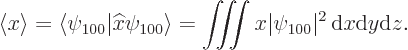
The po­si­tion co­or­di­nates $y$ and $z$ go the same way, and it fol­lows that the ex­pec­ta­tion value of po­si­tion is at $(x,y,z)$ $\vphantom0\raisebox{1.5pt}{$=$}$ (0,0,0); the ex­pec­ta­tion po­si­tion of the elec­tron is in nu­cleus.

In fact, all ba­sic en­ergy eigen­func­tions $\psi_{nlm}$ of the hy­dro­gen atom, like fig­ures 4.9, 4.10, 4.11, 4.12, as well as the com­bi­na­tion states 2p$_x$ and 2p$_y$ of fig­ure 4.13, have a sym­met­ric prob­a­bil­ity dis­tri­b­u­tion, and all have the ex­pec­ta­tion value of po­si­tion in the nu­cleus. (For the hy­brid states dis­cussed later, that is no longer true.)

But don’t re­ally ex­pect to ever find the elec­tron in the neg­li­gi­ble small nu­cleus! You will find it at lo­ca­tions that are on av­er­age one stan­dard de­vi­a­tion away from it. For ex­am­ple, in the ground state

$$\sigma_x=\sqrt{\langle(x-\left\langle{x}\right\rangle )^2\r... ...x^2 \vert\psi_{100}(x,y,z)\vert^2 { \rm d}x{\rm d}y {\rm d}z}$$

which is pos­i­tive since the in­te­grand is every­where pos­i­tive. So, the re­sults of $x$-​po­si­tion mea­sure­ments are un­cer­tain, even though they av­er­age out to the nom­i­nal po­si­tion $x$ $\vphantom0\raisebox{1.5pt}{$=$}$ 0. The neg­a­tive ex­per­i­men­tal re­sults for $x$ av­er­age away against the pos­i­tive ones. The same is true in the $y$ and $z$ di­rec­tions. Thus the ex­pec­ta­tion po­si­tion be­comes the nu­cleus even though the elec­tron will re­ally never be found there.

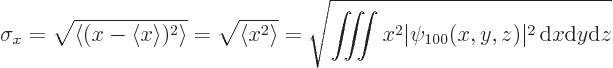
If you ac­tu­ally do the in­te­gral above, (it is not dif­fi­cult in spher­i­cal co­or­di­nates,) you find that the stan­dard de­vi­a­tion in $x$ equals the Bohr ra­dius. So on av­er­age, the elec­tron will be found at an $x$-​dis­tance equal to the Bohr ra­dius away from the nu­cleus. Sim­i­lar de­vi­a­tions will oc­cur in the $y$ and $z$ di­rec­tions.

The ex­pec­ta­tion value of lin­ear mo­men­tum in the ground state can be found from the lin­ear mo­men­tum op­er­a­tor ${\widehat p}_x$ $\vphantom0\raisebox{1.5pt}{$=$}$ $\hbar\partial$$\raisebox{.5pt}{$/$}$​${\rm i}\partial{x}$:

$$\langle p_x\rangle = \langle \psi_{100}\vert{\widehat p}_x... ...al\frac12\psi_{100}^2}{\partial x} { \rm d}x{\rm d}y {\rm d}z$$

This is again zero, since dif­fer­en­ti­a­tion turns a sym­met­ric func­tion into an an­ti­sym­met­ric one, one which changes sign be­tween neg­a­tive and cor­re­spond­ing pos­i­tive po­si­tions. Al­ter­na­tively, just per­form in­te­gra­tion with re­spect to x, not­ing that the wave func­tion is zero at in­fin­ity.

More gen­er­ally, the ex­pec­ta­tion value for lin­ear mo­men­tum is zero for all the en­ergy eigen­func­tions; that is a con­se­quence of Ehren­fest's the­o­rem cov­ered in chap­ter 7.2.1. The stan­dard de­vi­a­tions are again nonzero, so that lin­ear mo­men­tum is un­cer­tain like po­si­tion is.

All these ob­ser­va­tions carry over in the same way to the eigen­func­tions $\psi_{n_xn_yn_z}$ of the har­monic os­cil­la­tor. They too all have the ex­pec­ta­tion val­ues of po­si­tion at the ori­gin, in other words in the nu­cleus, and the ex­pec­ta­tion lin­ear mo­menta equal to zero.

If com­bi­na­tions of en­ergy eigen­func­tions are con­sid­ered, it changes. Such com­bi­na­tions may have non­triv­ial ex­pec­ta­tion po­si­tions and lin­ear mo­menta. A dis­cus­sion will have to wait un­til chap­ter 7.

Key Points

$\begin{picture}(15,5.5)(0,-3) \put(2,0){\makebox(0,0){\scriptsize\bf0}} \put(12... ...\thicklines \put(3,0){\line(1,0){12}}\put(11.5,-2){\line(1,0){3}} \end{picture}$

Ex­am­ples of def­i­nite and un­cer­tain quan­ti­ties were given for ex­am­ple wave func­tions.

$\begin{picture}(15,5.5)(0,-3) \put(2,0){\makebox(0,0){\scriptsize\bf0}} \put(12... ...\thicklines \put(3,0){\line(1,0){12}}\put(11.5,-2){\line(1,0){3}} \end{picture}$

A quan­tity has a def­i­nite value when the wave func­tion is an eigen­func­tion of the op­er­a­tor cor­re­spond­ing to that quan­tity.