13.1 The Elec­tro­mag­netic Hamil­ton­ian

This sec­tion de­scribes very ba­si­cally how elec­tro­mag­net­ism fits into quan­tum me­chan­ics. How­ever, elec­tro­mag­net­ism is fun­da­men­tally rel­a­tivis­tic; its car­rier, the pho­ton, read­ily emerges or dis­ap­pears. To de­scribe elec­tro­mag­netic ef­fects fully re­quires quan­tum elec­tro­dy­nam­ics, and that is far be­yond the scope of this text. (How­ever, see ad­denda {A.15} and {A.23} for some of the ideas.)

In clas­si­cal elec­tro­mag­net­ics, the force on a par­ti­cle with charge $q$ in a field with elec­tric strength $\skew3\vec{\cal E}$ and mag­netic strength $\skew2\vec{\cal B}$ is given by the Lorentz force law

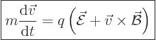$$\fbox{$\displaystyle m \frac{{\rm d}\vec v}{{\rm d}t} = q... ...kew3\vec{\cal E}+ \vec v\times \skew2\vec{\cal B}\right) $} %$$ (13.1)

where $\vec{v}$ is the ve­loc­ity of the par­ti­cle and for an elec­tron, the charge is $q$ $\vphantom0\raisebox{1.5pt}{$=$}$ $\vphantom{0}\raisebox{1.5pt}{$-$}$$e$.

Un­for­tu­nately, quan­tum me­chan­ics uses nei­ther forces nor ve­loc­i­ties. In fact, the ear­lier analy­sis of atoms and mol­e­cules in this book used the fact that the elec­tric field is de­scribed by the cor­re­spond­ing po­ten­tial en­ergy $V$, see for ex­am­ple the Hamil­ton­ian of the hy­dro­gen atom. The mag­netic field must ap­pear dif­fer­ently in the Hamil­ton­ian; as the Lorentz force law shows, it cou­ples with ve­loc­ity. You would ex­pect that still the Hamil­ton­ian would be rel­a­tively sim­ple, and the sim­plest idea is then that any po­ten­tial cor­re­spond­ing to the mag­netic field moves in to­gether with mo­men­tum. Since the mo­men­tum is a vec­tor quan­tity, then so must be the mag­netic po­ten­tial. So, your sim­plest guess would be that the Hamil­ton­ian takes the form

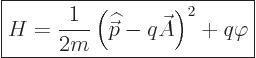$$\fbox{$\displaystyle H = \frac{1}{2m}\left({\skew 4\widehat{\skew{-.5}\vec p}}- q \skew3\vec A\right)^2 + q \varphi $} %$$ (13.2)

where $\varphi$ $\vphantom0\raisebox{1.5pt}{$=$}$ $V$$\raisebox{.5pt}{$/$}$​$q$ is the elec­tric po­ten­tial and $\skew3\vec A$ is the mag­netic vec­tor po­ten­tial. And this sim­plest guess is in fact right.

The re­la­tion­ship be­tween the vec­tor po­ten­tial $\skew3\vec A$ and the mag­netic field strength $\skew2\vec{\cal B}$ will now be found from re­quir­ing that the clas­si­cal Lorentz force law is ob­tained in the clas­si­cal limit that the quan­tum un­cer­tain­ties in po­si­tion and mo­men­tum are small. In that case, ex­pec­ta­tion val­ues can be used to de­scribe po­si­tion and ve­loc­ity, and the field strengths $\skew3\vec{\cal E}$ and $\skew2\vec{\cal B}$ will be con­stant on the small quan­tum scales. That means that the de­riv­a­tives of $\varphi$ will be con­stant, (since $\skew3\vec{\cal E}$ is the neg­a­tive gra­di­ent of $\varphi$), and pre­sum­ably the same for the de­riv­a­tives of $\skew3\vec A$.

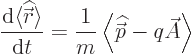
Now ac­cord­ing to chap­ter 7.2, the evo­lu­tion of the ex­pec­ta­tion value of po­si­tion is found as

$$\frac{{\rm d}\langle {\skew 2\widehat{\skew{-1}\vec r}}\ran... ...\langle \frac{{\rm i}}{\hbar} [H,{\skew0\vec r}] \right\rangle$$

Work­ing out the com­mu­ta­tor with the Hamil­ton­ian above, {D.71}, you get,

$$\frac{{\rm d}\langle {\skew 2\widehat{\skew{-1}\vec r}}\ran... ...\skew 4\widehat{\skew{-.5}\vec p}}- q\skew3\vec A\right\rangle$$

This is un­ex­pected; it shows that ${\skew 4\widehat{\skew{-.5}\vec p}}$, i.e. $\hbar\nabla$$\raisebox{.5pt}{$/$}$​${\rm i}$, is no longer the op­er­a­tor of the nor­mal mo­men­tum $m\vec{v}$ when there is a mag­netic field; ${\skew 4\widehat{\skew{-.5}\vec p}}-q\skew3\vec A$ gives the nor­mal mo­men­tum. The mo­men­tum rep­re­sented by ${\skew 4\widehat{\skew{-.5}\vec p}}$ by it­self is called “canon­i­cal” mo­men­tum to dis­tin­guish it from nor­mal mo­men­tum:

The canon­i­cal mo­men­tum $\hbar\nabla$$\raisebox{.5pt}{$/$}$​${\rm i}$ only cor­re­sponds to nor­mal mo­men­tum if there is no mag­netic field in­volved.

(Ac­tu­ally, it was not that un­ex­pected to physi­cists, since the same hap­pens in the clas­si­cal de­scrip­tion of elec­tro­mag­net­ics us­ing the so-called La­grangian ap­proach, chap­ter 1.3.2.)

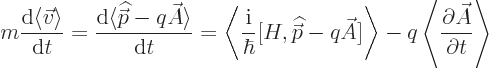
Next, New­ton’s sec­ond law says that the time de­riv­a­tive of the lin­ear mo­men­tum $m\vec{v}$ is the force. Since ac­cord­ing to the above, the lin­ear mo­men­tum op­er­a­tor is ${\skew 4\widehat{\skew{-.5}\vec p}}-q\skew3\vec A$, then

$$m \frac{{\rm d}\langle\vec v\rangle}{{\rm d}t} = \frac{{\... ...\langle \frac{\partial \skew3\vec A}{\partial t} \right\rangle$$

The ob­jec­tive is now to en­sure that the right hand side is the cor­rect Lorentz force (13.1) for the as­sumed Hamil­ton­ian, by a suit­able de­f­i­n­i­tion of $\skew2\vec{\cal B}$ in terms of $\skew3\vec A$.

Af­ter a lot of grind­ing down com­mu­ta­tors, {D.71}, it turns out that in­deed the Lorentz force is ob­tained,

$$m \frac{{\rm d}\langle \vec v \rangle}{{\rm d}t} = q \left... ...al E}+ \langle \vec v \rangle \times \skew2\vec{\cal B}\right)$$

pro­vided that:

$$\fbox{$\displaystyle \skew3\vec{\cal E}= -\nabla \varphi -... ... \qquad \skew2\vec{\cal B}= \nabla \times \skew3\vec A $} %$$ (13.3)

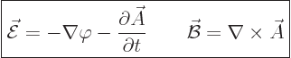
So the mag­netic field is found as the curl of the vec­tor po­ten­tial $\skew3\vec A$. And the elec­tric field is no longer just the neg­a­tive gra­di­ent of the scalar po­ten­tial $\varphi$ if the vec­tor po­ten­tial varies with time.

These re­sults are not new. The elec­tric scalar po­ten­tial $\varphi$ and the mag­netic vec­tor po­ten­tial $\skew3\vec A$ are the same in clas­si­cal physics, though they are a lot less easy to guess than done here. More­over, in clas­si­cal physics they are just con­ve­nient math­e­mat­i­cal quan­ti­ties to sim­plify analy­sis. In quan­tum me­chan­ics they ap­pear as cen­tral to the for­mu­la­tion.

And it can make a dif­fer­ence. Sup­pose you do an ex­per­i­ment where you pass elec­tron wave func­tions around both sides of a very thin mag­net: you will get a wave in­ter­fer­ence pat­tern be­hind the mag­net. The clas­si­cal ex­pec­ta­tion is that this in­ter­fer­ence pat­tern will be in­de­pen­dent of the mag­net strength: the mag­netic field $\skew2\vec{\cal B}$ out­side a very thin and long ideal mag­net is zero, so there is no force on the elec­tron. But the mag­netic vec­tor po­ten­tial $\skew3\vec A$ is not zero out­side the mag­net, and Aharonov and Bohm ar­gued that the in­ter­fer­ence pat­tern would there­fore change with mag­net strength. So it turned out to be in ex­per­i­ments done sub­se­quently. The con­clu­sion is clear; na­ture re­ally goes by the vec­tor po­ten­tial $\skew3\vec A$ and not the mag­netic field $\skew2\vec{\cal B}$ in its ac­tual work­ings.