|
|
|
To: 8.4 Summary |
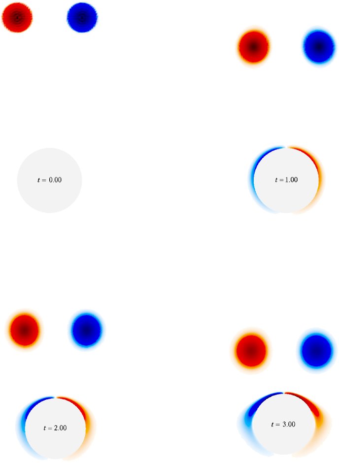
Vortex interaction with solid walls is an important basic issue of practical interest [73]. For example, a current issue of great concern for fighter planes is that conventional computations greatly diffuse separated vorticity coming from the wings, causing erroneous interactions with the tail surfaces.
As a simple model problem for this phenomenon, we computed the propagation
of a vortex-pair towards the surface of a cylinder.
This provides an elementary example of the power of a mesh-free method,
see figure 8.38. We will nondimensionalize the problem with
the diameter ![]() of the cylinder and
of the cylinder and
![]() , where
, where
![]() is the circulation of the incoming vortices. The Reynolds
number, defined as
is the circulation of the incoming vortices. The Reynolds
number, defined as
![]() , was taken to be 500. We
took the vortices initially one diameter apart, hence their initial drift
velocity is approximately unity in our normalizations. Initially the
vortices are 2.5 diameters away from the center of the cylinder, and for
simplicity we took their initial vorticity profiles to be those of point
vortices that have already diffused out for a nondimensional time interval
, was taken to be 500. We
took the vortices initially one diameter apart, hence their initial drift
velocity is approximately unity in our normalizations. Initially the
vortices are 2.5 diameters away from the center of the cylinder, and for
simplicity we took their initial vorticity profiles to be those of point
vortices that have already diffused out for a nondimensional time interval
![]() .
.
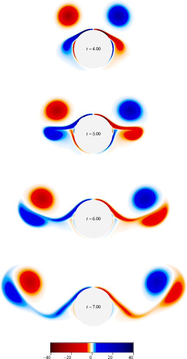
Figure 8.38 shows the evolution of the vorticity field; the evolution of the separated vorticity field agrees with existing experimental and computational data for similar flows [39,168,244,250]. Initially, when the vortex pair is still sufficiently far away, the boundary layer on the cylinder surface develops similar to that on an impulsively translated cylinder. When the vortex pair approaches closer to the cylinder, the boundary layer separates and rolls up into a vortex (secondary vortex); this secondary vortex deflects the oncoming primary vortex.
 |
 |
Figure 8.40 shows the location of the vortex center ![]() or centroid
of the approaching vortex in one half plane at different times.
The vortex path is similar to that of Yamada, Yamabe, Itoh
& Hayashi [250],
showing the `rebounding' effect.
Figure 8.41 shows that the circulation of the
secondary vortex is of the same order as the primary vortex.
or centroid
of the approaching vortex in one half plane at different times.
The vortex path is similar to that of Yamada, Yamabe, Itoh
& Hayashi [250],
showing the `rebounding' effect.
Figure 8.41 shows that the circulation of the
secondary vortex is of the same order as the primary vortex.
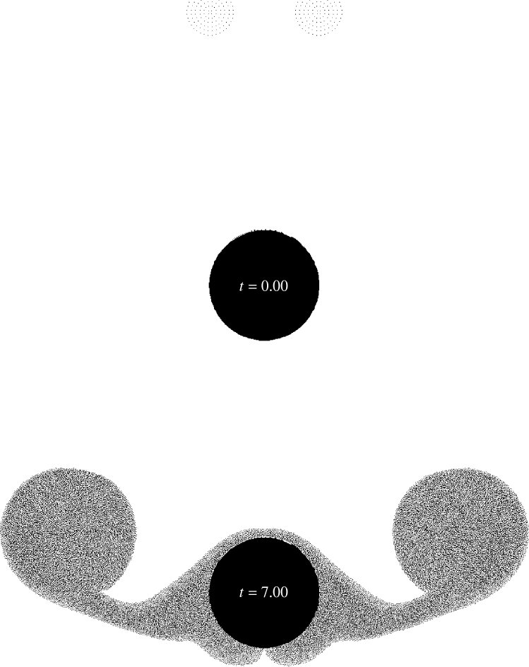
Standard numerical procedures experience various difficulties with this flow. For example, a very large single mesh could be defined to enclose all of this flow. But to maintain high resolution both in the incoming vortices and near the wall, this would require large amounts of mesh points. A better choice would seem to be to use multiple meshes, hence giving each part of the flow its own mesh. But such a procedure would experience complications in logic at the later times when the vorticity regions meet and join.
Instead, in our mesh-free procedure we merely placed two set of computational vortices at the locations of the incoming physical vortices. There is no need to structure or order these in our scheme. Except for this simple incorporation of the initial conditions, we ran our scheme for the circular cylinder of section 8.2 completely unchanged. Our wall boundary condition treatment (section 6.3) automatically starts adding vortices at the wall because of the slip velocity induced by the incoming vortices. Our vorticity redistribution method automatically extends the vortices out away from the wall when the vorticity diffuses there. When the different regions of vorticity meet, the vortices of one region automatically begin to use vortices of another region, whenever it is convenient. At all times, the computational vortices remain restricted to only the regions where we need them. This shown in figure 8.42. Such an excellent adaptive resolution of separated vorticity fields would be very difficult to achieve in mesh-based computations.