|
|
|
To: 8.2.3 Velocity field |
In this subsection we show that our computed streamlines do indeed predict the flow features observed in the experimental results very accurately.
 |
 |
 |
 |
 |
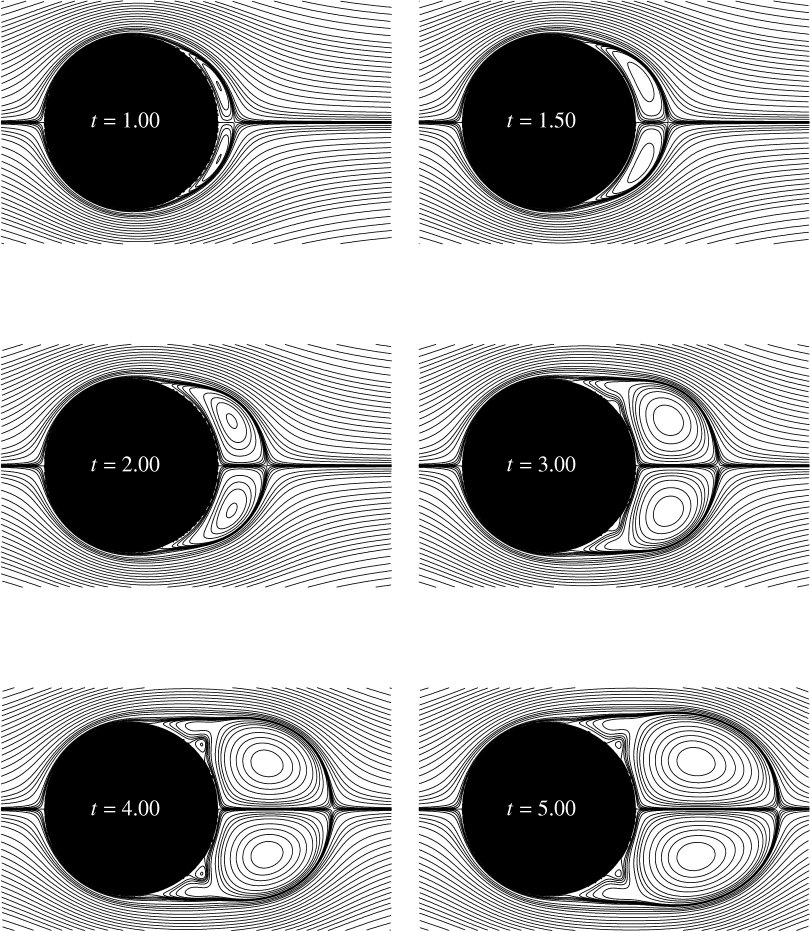
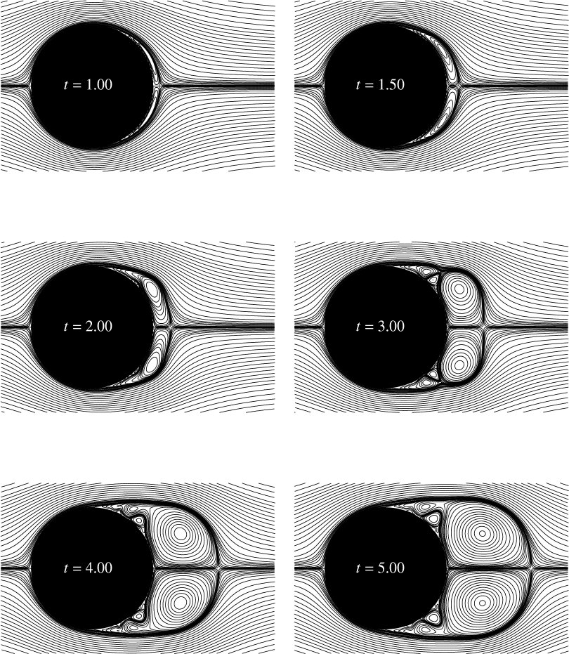
Computed streamlines are shown
in figures 8.4, 8.6 and 8.8
for ![]() , 3,000, and 9,500 respectively.
Note that the fluid comes from the left of the cylinder.
The characteristic feature
is the presence of a large recirculating flow region
of closed streamlines behind the cylinder.
The streamwise length of this recirculating region,
also known as the wake length [29], grows in time.
The wake length at any fixed time is smaller
for increasing Reynolds number.
, 3,000, and 9,500 respectively.
Note that the fluid comes from the left of the cylinder.
The characteristic feature
is the presence of a large recirculating flow region
of closed streamlines behind the cylinder.
The streamwise length of this recirculating region,
also known as the wake length [29], grows in time.
The wake length at any fixed time is smaller
for increasing Reynolds number.
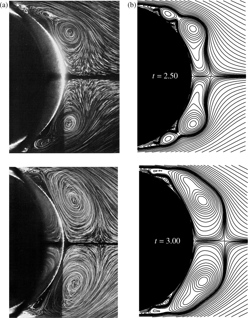
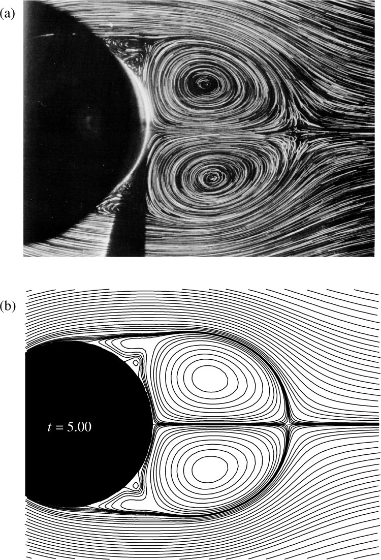
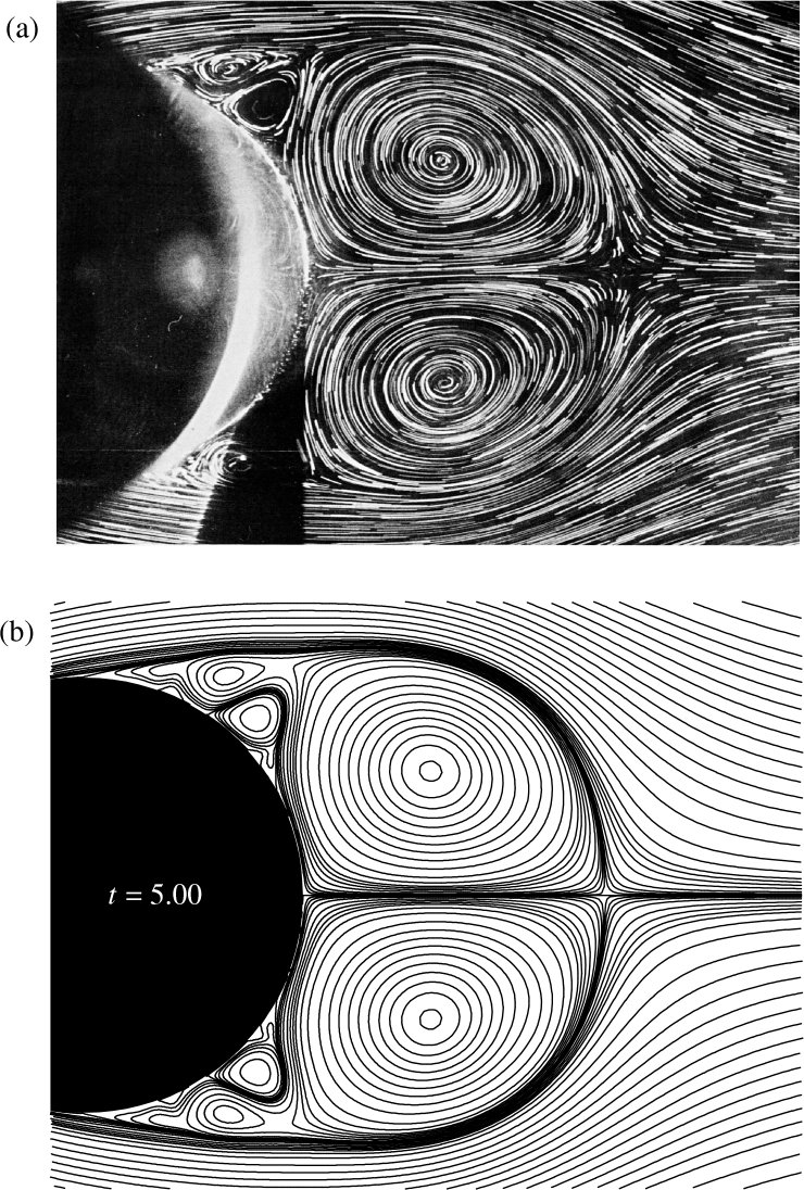
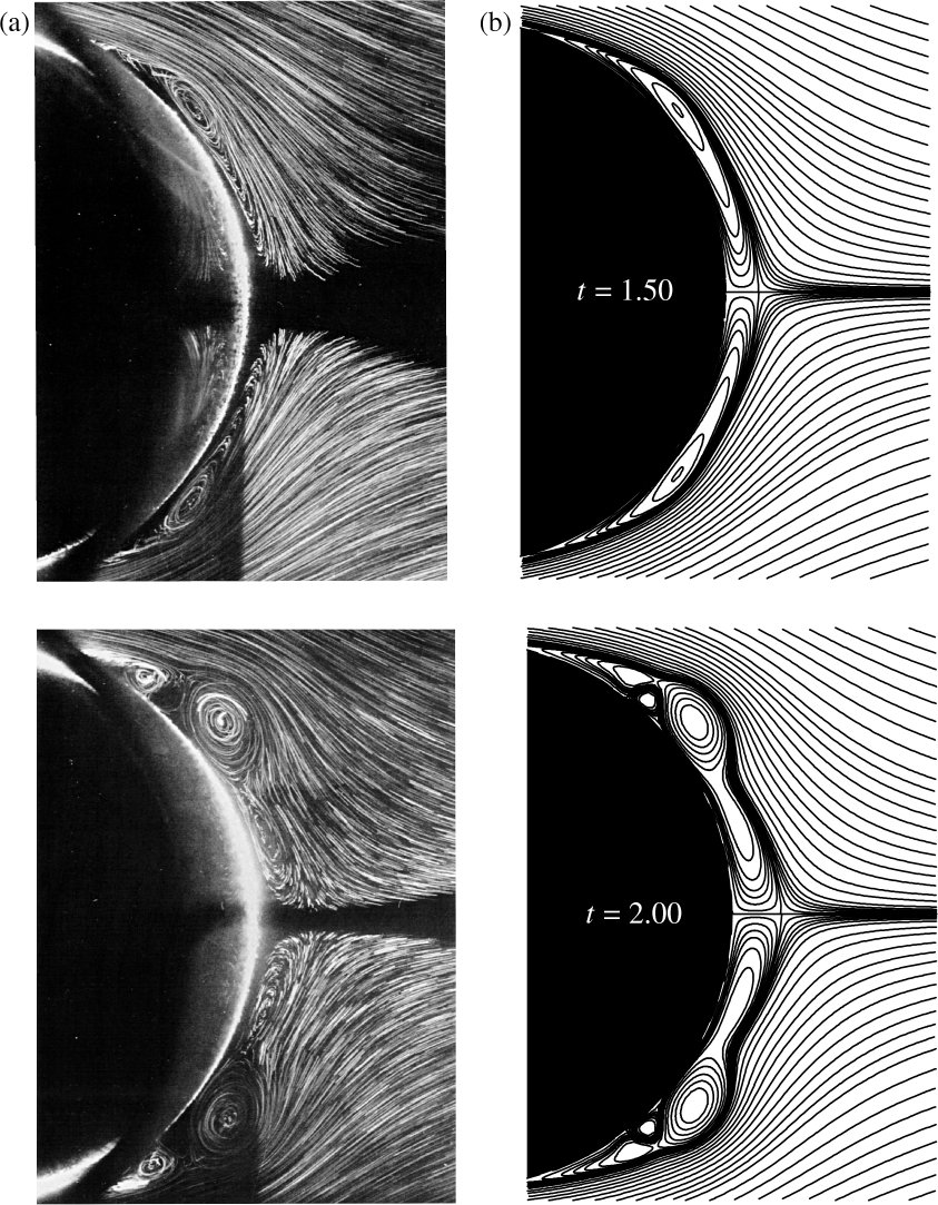
A comparison of our computed streamlines with those obtained in the
experiment
of Bouard & Coutanceau [29] is shown
in figures 8.5, 8.7, and 8.8
for ![]() , 3,000, and 9,500 respectively.
Our streamlines in the large recirculating flow region behind the
cylinder are in good visual agreement with those of the experiment.
In addition to this large recirculating flow region,
a number of smaller recirculating flow regions along the rear half
of the cylinder surface seen in the experiment are also observed in
our computations. As shown by Lecointe &
Piquet [123],
some of the earlier finite difference computations were not able to
reproduce these smaller recirculating flow regions.
, 3,000, and 9,500 respectively.
Our streamlines in the large recirculating flow region behind the
cylinder are in good visual agreement with those of the experiment.
In addition to this large recirculating flow region,
a number of smaller recirculating flow regions along the rear half
of the cylinder surface seen in the experiment are also observed in
our computations. As shown by Lecointe &
Piquet [123],
some of the earlier finite difference computations were not able to
reproduce these smaller recirculating flow regions.
For completeness, we now give the parameters of our figures
8.4 through 8.8.
Using the usual left-handed ![]() coordinate system with origin at the
center of the cylinder, the figure dimensions and streamline
contour values are as follows:
in figure 8.4 for
coordinate system with origin at the
center of the cylinder, the figure dimensions and streamline
contour values are as follows:
in figure 8.4 for ![]() and
figure 8.6 for
and
figure 8.6 for ![]() ,
, ![]() has the range [-1.5,3.0] and
has the range [-1.5,3.0] and
![]() has the range [-1.4,1.4];
in both these figures, the streamline contour values are
0,
has the range [-1.4,1.4];
in both these figures, the streamline contour values are
0, ![]() {0.001, 0.0025, 0.005, 0.01, 0.03, 0.05, 0.07, 0.1, 0.15,
0.2, 0.25, 0.3, 0.35, 0.4, 0.45, 0.5, 0.55, 0.6, 0.65, 0.7, 0.75,
0.8, 0.875, 0.95, 1.025, 1.10, 1.175, and 1.25 }.
In figure 8.5 for
{0.001, 0.0025, 0.005, 0.01, 0.03, 0.05, 0.07, 0.1, 0.15,
0.2, 0.25, 0.3, 0.35, 0.4, 0.45, 0.5, 0.55, 0.6, 0.65, 0.7, 0.75,
0.8, 0.875, 0.95, 1.025, 1.10, 1.175, and 1.25 }.
In figure 8.5 for ![]() ,
, ![]() has the range [-0.54,3.75],
has the range [-0.54,3.75],
![]() has the range [-1.63,1.63], and the streamline values are same as above.
In figures 8.7 for
has the range [-1.63,1.63], and the streamline values are same as above.
In figures 8.7 for ![]() ,
,
![]() has the range [-0.16,3.10],
has the range [-0.16,3.10],
![]() has the range [-1.26,1.26], and the streamline values are same as above.
In figure 8.8 for
has the range [-1.26,1.26], and the streamline values are same as above.
In figure 8.8 for ![]() ,
,
![]() has the range [-0.25,1.75] and
has the range [-0.25,1.75] and
![]() has the range [-1.05,1.05]; the streamline values are
0,
has the range [-1.05,1.05]; the streamline values are
0, ![]() {0.001, 0.003, 0.005, 0.007, 0.01, 0.015, 0.027, 0.04,
0.06, 0.08, 0.1, 0.125, 0.15, 0.18, 0.21, 0.24, 0.27, 0.3, 0.35,
0.4, 0.45, 0.5, 0.55, 0.6, 0.65, and 0.7 }.
{0.001, 0.003, 0.005, 0.007, 0.01, 0.015, 0.027, 0.04,
0.06, 0.08, 0.1, 0.125, 0.15, 0.18, 0.21, 0.24, 0.27, 0.3, 0.35,
0.4, 0.45, 0.5, 0.55, 0.6, 0.65, and 0.7 }.
In view of the fact that an impulsive start cannot be exactly reproduced experimentally, the agreement between our computation and the experimental data for the streamlines is excellent. However, many other computations, [40,117,134] for example, have also shown such good visual agreement between their computed streamline patterns and those of the experiments. A much stronger test is a comparison of higher order derivatives of the streamfunction, such as the velocity and vorticity fields, and the drag force on the cylinder for example. In the next subsection we compare our computed velocity field with those obtained from both experiments as well as other computations.