|
|
|
To: 8. Computation of Flows over Solid Walls |
To show that the redistribution method works equally well in
three dimensions, we consider two linear problems [202]:
diffusion of a pair of opposite vortex poles
and the Stokes flow (![]() ) due to a vortex ring in free space.
) due to a vortex ring in free space.
 |
Figure 7.19a shows the vorticity distribution of the vortex pair along the line connecting the vortices. Figure 7.19b shows the isovorticity contours in the right half of the plane containing the vortices. The solid lines are exact solutions and the dots are computed solutions; the solutions are in very good agreement. Our computations show that the circular symmetries in the solution are reproduced very well, even though the symmetries are not explicitly enforced.
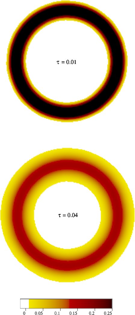
Figure 7.20 shows the vorticity field due to the diffusion of a vortex ring at two different times. It is seen that the mean thickness of the ring expands correctly as expected and also preserves the circular symmetry very well.
Hence, the results presented in this chapter show that the vorticity redistribution method can handle flows in free space accurately. In the next chapter we will apply the vorticity redistribution method to two-dimensional flows over solid walls.