 |
Leon van Dommelen
1/31/97
This document describes the Reynolds transport theorem, which converts the laws you saw previously in your physics, thermodynamics, and chemistry classes to laws in fluid mechanics. The laws of physics look somewhat different in fluid mechanics, even though they are of course still exactly the same.
The difficulty is that your earlier classes always talked about a fixed quantity of fluid. For example, they told you that the mass of the fluid never changed (ignoring relativity effects). Also, Newton's second law said that the rate of change of the linear momentum of the fluid equals the total external force exerted on the fluid. And the first law of thermodynamics said that the total internal and kinetic energy of the fluid increases according to the work being done on the fluid and the heat being added to it. All these statements are only true of we consider a fixed quantity of fluid.
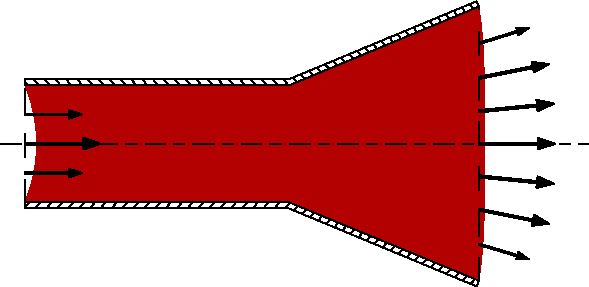
Fluid mechanics does not usually consider the same fluid at all times. For example, fluid mechanics may consider the flow through a pipe, such as maybe the funnel-shaped pipe below. The region within the shown pipe is fixed in space and is called a control volume. The fluid in a control volume changes when fluid flows in or out. In the pipe below, fluid enters one end of the pipe and leaves at the other end. The laws of physics do not directly apply to the pipe because the fluid in the pipe at one time is not the same fluid as at another time.
|
For most flows studied in fluid mechanics, in or outflow is common. A jet engine on a plane is another example. So is the flow around a vehicle such as a car or an airplane. Seen moving along with the vehicle; new fluid continuously enters the vicinity of the vehicle from upstream while fluid departs downstream. Gas flows out of a rocket.
For regions which contain different fluid at different times, the laws of physics, thermodynamics, and chemistry do not directly apply; they must be corrected for the entering and departing fluid. In fact, you already know from calculus and thermodynamics that derivatives may depend on what you keep constant.
As an example, consider the pipe flow shown in figure 1 at an
arbitrary time t0. One of the things physics tells you is that the
net force, call it ![]() , on the fluid inside the pipe gives you
the rate of change of linear momentum of the fluid. That means
that if the momentum of the fluid in the pipe at time t0 is
, on the fluid inside the pipe gives you
the rate of change of linear momentum of the fluid. That means
that if the momentum of the fluid in the pipe at time t0 is
![]() , then the momentum of this fluid at time
, then the momentum of this fluid at time ![]() will be
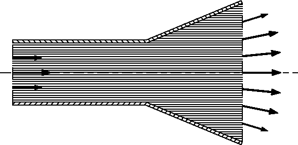
will be ![]() . In figure 2, the fluid
at time
. In figure 2, the fluid
at time ![]() is shown shaded; this fluid now has
is shown shaded; this fluid now has ![]() additional linear momentum.
additional linear momentum.
But what happens to the linear momentum in the pipe? In other
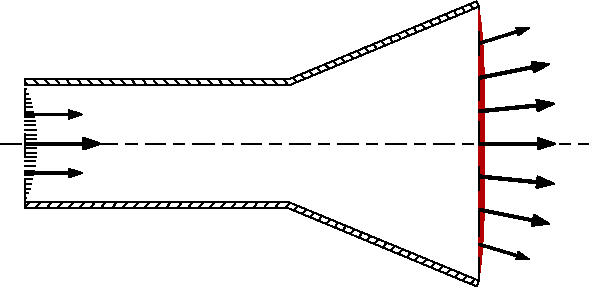
words, for the horizontally hatched region in figure 3? It has not
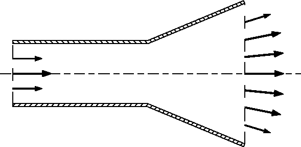
necessarily changed by ![]() . After all, the pipe now
contains some fluid which was not there before, shown as the hatched
strip in figure 4. The pipe has also lost some of its previous fluid,
shown as the shaded strip in figure 4. Mathematically, if we call the
linear momentum in the pipe
. After all, the pipe now
contains some fluid which was not there before, shown as the hatched
strip in figure 4. The pipe has also lost some of its previous fluid,
shown as the shaded strip in figure 4. Mathematically, if we call the
linear momentum in the pipe ![]() , the change of linear momentum
in the pipe,
, the change of linear momentum
in the pipe,
![]()
The trick is to add the momentum in the shaded strip (call it S) to the momentum in the pipe and to substract the momentum in the hatched strip (call it H). This gives us back the momentum in the fluid region, which we know. In short
![]()
A bit later we will show that the correction terms [momentum in S] - [momentum in H] can be written as a single integral over the entire outside surface A of the region within the pipe:
![]()
The bottom line is that conservation of linear momentum for a pipe, or any other fixed volume, takes the form:
| |
(1) |
If you look closer at the integral, you will see that it makes sense.
The outflow through an area element dA of the surface of the region
inside the pipe is obviously proportional to dA. It is clearly also
proportional to the component of the fluid velocity which is
normal to the area; motion in the direction of the surface does not
lead to in or outflow. And where the normal component of velocity
changes sign, we switch from inflow to outflow; the contribution to
the momentum equation then also changes sign as it should. The net
momentum outflow is also proportional to ![]() , which is the
linear momentum of the fluid per unit volume.
, which is the
linear momentum of the fluid per unit volume.
Now we will show that indeed the linear momentum in the two strips in
figure 4 can be written as the single integral over all of the surface
area of the control volume. In figure 5 we show a typical segment of
the outflow strip corresponding to an area element dA of the outside
surface of the control volume. We also show the local unit vector
![]() which is normal to area element dA. Using this vector, we
can find the component of the fluid velocity normal to dA as
which is normal to area element dA. Using this vector, we
can find the component of the fluid velocity normal to dA as ![]() .
.
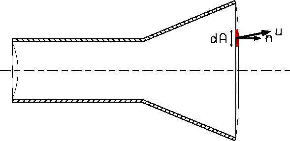 |
The thickness of the segment is equal to the
distance the fluid has travelled in the direction normal to dA, so
the thickness equals ![]() . The volume
dVS of this segment of the strip, given by the area dA times the
height, equals
. The volume
dVS of this segment of the strip, given by the area dA times the
height, equals
| |
(2) |
| |
(3) |
To get the total contribution, we simply integrate over all outside surface
areas of our control volume. The contribution of the inflow strip in figure
4 should be negative, but
since we always take the unit vector in the direction pointing
out of the control volume, this is automatically taken care off.
There is no in or outflow through the solid surface of the pipe itself, but
since ![]() is here zero, that too is automatic.
So we get the single integral over all the outside surface which we
wrote down earlier.
is here zero, that too is automatic.
So we get the single integral over all the outside surface which we
wrote down earlier.
How about conservation of mass? It is almost exactly the same story. If we take the change in the mass M inside the control volume and add to it the mass in the shaded strip in figure 4 and substract the mass in the hatched strip, we get the change in mass in the fluid region of figure 2;
![]()
| |
(4) |
For the equation for the energy we take the change in
the energy E inside the control volume and correct for the energy in the
strips in figure 4. This gives the change in energy for the fluid which
equals the work ![]() done on the fluid and
the heat
done on the fluid and
the heat ![]() added to it:
added to it:
![]()
| |
(5) |
It is clear that we can apply this same procedure to any other quantity in the fluid for which we know a conservation law. It should also not be very difficult to modify the above formulas in case the boundary of control volume itself also moves. For example, suppose the pipe of figure 1 is not rigidly suspended but vibrates horizontally?
Some additional notes. First, note that the work term in the energy equation is still the work done on the fluid. For example, do not think that the pressure force on the exit surface of the pipe in figure 1 does not perform work since the exit is fixed. The two left-hand-side terms in equation (5) together are simply the time derivative of the energy of the fluid. And we therefor need the work done on the phsyical fluid, not on the imaginary control volume. So we need, among others, the work done by the pressure forces on the right hand fluid boundary between figures 1 and 2.
Next, note that the mass M, momentum ![]() , and energy E in the
control volume can be found by integrating the mass, momentum,
and energy per unit volume over the volume:
, and energy E in the
control volume can be found by integrating the mass, momentum,
and energy per unit volume over the volume:
![]()
![]()
![]()
The approach to fluid mechanics which uses prescribed spatial regions or positions is called a Eulerian description after the mathematician Euler. Our pipe can be considered a Eulerian region. On the other hand, a description using given regions or points of fluid is called a Lagrangian description after Euler's contemporary Jean-Louis Lagrange. The fluid region shown as shaded in figure 2 is the Lagrangian region L that coincided with the Eulerian control volume V at time t0. The combined left hand sides in equations (1), (4), and (5) are simply the time derivatives of this Lagrangian fluid region L:
![]()
![]()
![]()
One other thing. So far we have only shown how derivatives of
regions fixed in space can be converted to derivatives of regions
of fluids by adding surface integrals. Now we want to examine how we
can convert partial time derivatives for points fixed in space
to time derivatives for points of fluid. For example, the
acceleration of the fluid, ![]() , is the Lagrangian time derivative of
the velocity keeping the fluid point constant. However, if
we have computed or measured a velocity field in Eulerian form as a
function
, is the Lagrangian time derivative of
the velocity keeping the fluid point constant. However, if
we have computed or measured a velocity field in Eulerian form as a
function ![]() , it will be the partial
derivative
, it will be the partial
derivative ![]() keeping the spatial position
constant which is immediately available. How do we find the time
derivative
keeping the spatial position
constant which is immediately available. How do we find the time
derivative ![]() following the fluid? The answer is simply
the chain rule of differentiation. For any function f,
following the fluid? The answer is simply
the chain rule of differentiation. For any function f,
![]()
| |
(6) |
| |
(7) |